Heisenberg’s uncertainty principle states that the position and momentum of a particle cannot be determined simultaneously with unlimited precision.
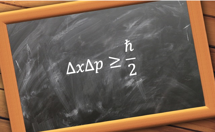
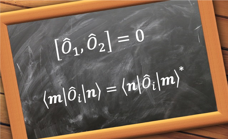
The uncertainty not only applies to the position and momentum of a particle, but to any pair of complementary observables, e.g. energy and time. In general, the uncertainty principle is expressed as:
where and
are Hermitian operators and
and
are their respective observables.
The derivation of eq12 involves the following:
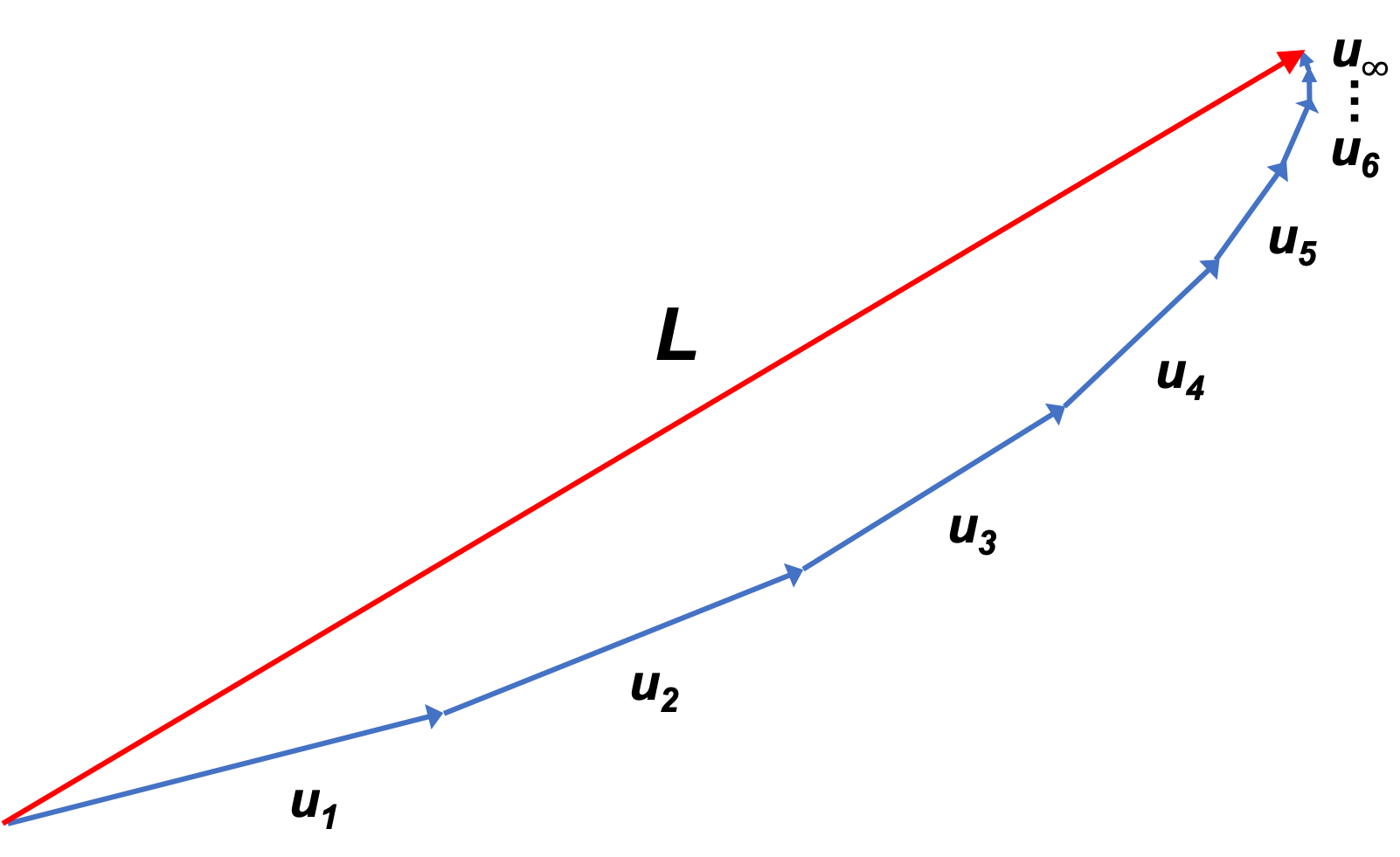
- Deriving the Schwarz inequality
- Proving the inequality
- Showing that
Step 1
Let
where and
are arbitrary square integrable wavefunctions and
is an arbitrary scalar.
Since
Expanding eq13, we have
Since is an arbitrary scalar, substituting
and
in eq15 gives:
Substituting eq14 in the above equation and rearranging yields . Since
Eq16 is called the Schwarz Inequality.
Step 2
Let and
, where
is normalised, and
and
are Hermitian operators, which implies that
and
are also Hermitian operators (see this article for proof). The variance of the observable of
is
Note that the 2nd last equality uses the property of Hermitian operators (see eq36). Similarly,
Substituting eq17 and eq18 in eq16 results in
Let where
. So,
. Since
, we have
, which is
Substituting eq19 in eq20 gives
Next, we have
Similarly,
Substituting eq22 and eq23 in eq21 yields
Step 3
We have used eq37 for the 2nd equality and eq35 for the 3rd equality. Substituting eq25 in one of the in eq24 results in
Therefore,
which is eq12, the general form of the uncertainty principle.
For, the observable pair of position and momentum
, we have
Since