Category: Advanced Chemistry

The relativistic energy–momentum relation describes how an object’s total energy is determined by both its momentum (motion through space) and its invariant mass (rest mass).

To derive the relation, consider the relativistic definition of momentum in terms of proper time,

where is the rest mass and  is the proper time measured by a clock moving with the object.

According to time dilation, , where . Since the object’s velocity in the observer’s frame is , we have . Therefore,

From the definition of work, , or equivalently, , since and . Differentiating eq254a throughout yields

 

 

Substituting and into results in , or its integrated form

where is a constant.

To satisfy Einstein’s mass-energy equivalence relation , where is the rest mass, eq254b must give when . Since at , this requires . Thus, eq254b becomes

From eq254a, . Substracting this from the square of eq254c gives

Since ,

Therefore,

This is the relativistic energy–momentum relation.

Interestngly, has two solutions. The negative-energy solution seems problematic because ordinary particles are expected to have positive energy. However, it cannot consistently be discarded. This eventually led Paul Dirac to interpret the negative solution as corresponding to antiparticles.

 

Next article: Why does a current flowing through a wire generate a magnetic field

Previous article: The Twin Paradox

Content page of quantum mechanics

Content page of advanced chemistry

Main content page

The Bose–Einstein distribution describes how indistinguishable bosons are distributed among available energy states at thermal equilibrium.

To derive the Bose–Einstein distribution, consider a system of fixed-volume containing bosons occupying discrete single-particle energy levels , each with degeneracy , with no restriction on the number of bosons that can occupy a single state. The total number of bosons and the total energy of the system are

where

Replicas of this system form a microcanonical ensemble, meaning that only configurations with the same fixed and are allowed.

Since any number of bosons can occupy the same single-particle state, the number of ways to place bosons among the ​ degenerate states at energy is given by the stars-and-bars result:

For example, if two bosons occupy three degenerate states (), the possible occupation configurations are 200, 020, 002, 110, 101, or 011. Thus, there are six possible microstates, consistent with

It follows that the total number of microstates corresponding to a particular configuration is

For macroscopic systems, distinct single-particle energy levels are often extremely closely spaced. Consequently, many distinct energy levels can fall within a small energy interval. For the purposes of counting, these closely spaced levels may be treated as approximately degenerate, so that the interval contains a very large number of approximately degenerate single-particle states. Taking the natural logarithm of eq34 and substituting eq33 gives:

where  because  is large.

Using Stirling’s approximation. where ,  yields:

The possible configurations that define the microcanonical ensemble are restricted by eq31 and eq32. For example, the configurations and generally have different total energies and therefore cannot both belong to the same microcanonical ensemble. However, different configurations can have the same total energy and therefore can belong to the same microcanonical ensemble (see above diagram for an illustration). In such cases, all microstates corresponding to the allowed configurations satisfying the fixed  and constraints are equally probable. The most probable equilibrium configuration is therefore the one with the largest number of ways of achieving it, i.e. the one whose (or ) is maximal.

The total differential of is:

Hence, we want to solve for . With reference to Step 2 of the derivation of the Boltzmann distribution using the Lagrange method of undetermined multipliers, eq36 becomes:

where we have chosen minus signs for the 2^nd and 3^rd terms for convenience.

Since varies independently, eq37 holds only if each coefficient is zero:

Substituting eq35 into eq38, and noting that does not depend on , gives:

where we have changed the summation index from to in eq39 to distinguish the summation variable from the differentiation variable.

All terms in the summation of eq39 goes to zero except when . So,

Carrying out the differentiation and rearranging the result yields:

As mentioned above, is the number of bosons occupying the energy level . To transform eq40 into a probability distribution, we write:

where is the average or expected occupation number per degenerate state at energy . Thus, gives the total number of bosons occupying .

Substituting eq41 into eq40 gives:

The evaluation of the Lagrange multipliers and  proceeds in exactly the same way as for the Fermi-Dirac distribution, resulting in and . Therefore,

which is the Bose–Einstein distribution function.

For bosons, the chemical potential must satisfy , where is the lowest single-particle energy level. This condition ensures that the denominator in eq43 does not become negative or zero. In particular, when the ground-state energy is chosen to be zero (), the chemical potential satisfies . As approaches the ground-state energy from below (), the occupation of the lowest-energy state can become extremely large because

This behaviour is associated with Bose–Einstein condensation, in which a macroscopic number of bosons can occupy the lowest-energy quantum state.

For photons , the situation is slightly different. Although photons are bosons, their number is not conserved in thermal equilibrium because they can be freely created and absorbed through interactions with matter, e.g. . The chemical potential of a species is defined as the change in Gibbs free energy with respect to the change in the number of particles of that species , while the temperature, pressure and numbers of all other species are held constant: . Since is a minimum at equilibrium, if is free to vary. If is constrained and not free to vary, then may or may not be zero. Consequently, the chemical potential of photons is always zero at thermodynamic equilibrium, and eq43 becomes

which is the occupation factor underlying Planck’s blackbody radiation law, showing that blackbody radiation is fundamentally a quantum-statistical phenomenon.

 

Previous article: Fermi-Dirac distribution

Content page of statistical thermodynamics

Content page of advanced chemistry

Main content page

Maxwell’s fourth equation is a correction to Ampère’s law, stating that magnetic fields circulate around both electric currents and time-varying electric fields.

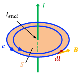
To understand why this correction was necessary, we first consider Ampère’s original law. From his experiments, Ampère observed that the circulation of the magnetic field around a closed loop is proportional to the electric current passing through the surface enclosed by the loop (see diagram above). This relationship is expressed mathematically by the line integral

where is an infinitesimal vector line element tangent to the closed path , whose magnitude is the differential path length and whose direction follows the chosen direction of integration around the loop, and is the proportionality constant known as the permeability of free space.

 

 

Eq30 is the integral form of Ampère’s law. While it accurately describes steady currents, it becomes inconsistent for situations involving time-varying electric fields, such as a charging capacitor.

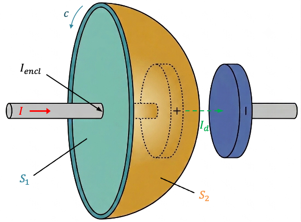
Consider a flat disc bounded by the closed loop . This surface intersects the wire perpendicularly to the left of the positive plate of the charging capacitor and is pierced by the conducting current (see diagram above). Therefore, according to Ampère’s law. A second dome-shaped surface , bounded by the same closed loop , bulges out between the capacitor plates. It passes between the plates but does not intersect the conducting wire. For this surface, , and Ampère’s law would predict . 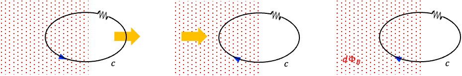However, the magnetic field surrounding the charging current does not disappear in the region between the capacitor plates. A magnetic needle placed near the gap still shows the same deflection as if it were placed near the conducting wire, indicating the presence of a magnetic field even though no conduction current flows across the gap. This contradicts the prediction of Ampère’s law.

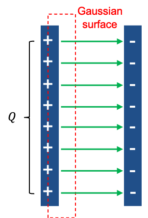
Maxwell resolved this inconsistency by introducing an effective current known as the displacement current flowing between the plates. To relate the electric field between the plates to the charge on either plate, we first note that joining the surfaces and forms a closed surface. This closed surface encloses part of the conducting wire as well as the positive capacitor plate, so it is not convenient for relating the electric field in the gap directly to the charge on the plate. Instead, we consider a new Gaussian surface that encloses only the charge on the inner surface of the positive capacitor plate (see diagram above). The left face of this Gaussian surface lies just inside the conducting plate, where , while its right face lies in the gap between the plates. Consequently, no electric flux passes through left face (), or the top and bottom faces (assuming fringing fields are negligible), and all the electric flux passes through the right face towards the negative plate.

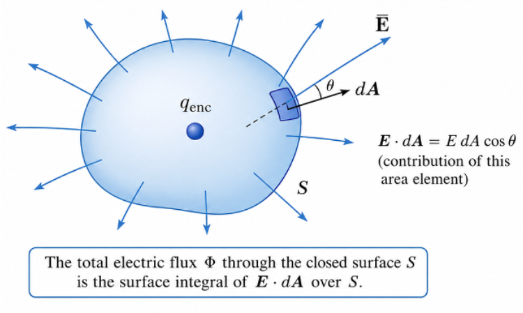
According to Gauss’s law, the electric flux through the Gaussian surface is . Differentiating this with respect to time gives:

Maxwell therefore defined the displacement current as . This leads to the integral form of Maxwell’s fourth equation (Ampère-Maxwell law):

For the surface , the enclosed current is entirely conduction current, so . For , no conduction current passes through the surface: . Thus both surfaces yield the same value of , removing the inconsistency in Ampère’s original law.

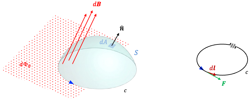
We can further express the conduction current through as the surface integral

where is the current density vector and is an infinitesimal area vector normal to the surface.

Differentiating the electric flux through the surface () with respect to time yields

where the time derivative may be moved inside the integral because the surface is assumed to be stationary.

Substituting eq32 and eq33 into eq31 results in:

Applying Stokes’ theorem gives:

Since this relation must hold for any arbitrary surface , the integrands must be equal at every point in space. Therefore,

which is the differential form of Maxwell’s fourth equation.

In a vacuum (free space), and eq34 becomes

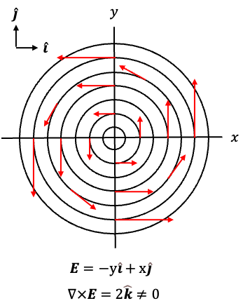
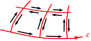
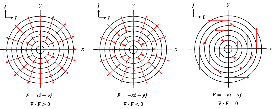
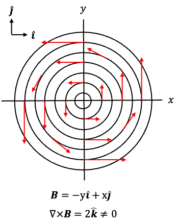
Circulating magnetic field lines are often illustrated using the vector function , or equivalently (see diagram above), where the field vectors are tangent to circles around the origin and point anticlockwise. For example, points upwards at , points left at , points downwards at , and points right at . Since the curl of  is given by

it is non-zero and points in the positive -direction. By the right-hand rule, this corresponds to positive (anticlockwise) circulation of the field in the -plane. Therefore, eq35 states that a time-varying electric field produces a circulating magnetic field .

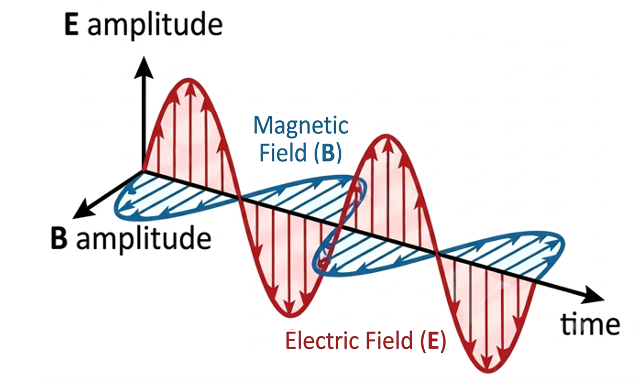
Notably, the curl of is itself a vector: . If the electric field oscillates with time, then its time derivative oscillates as well. According to eq35, the curl of the magnetic field then oscillates with time, causing the vector to oscillate. The magnetic field must, in turn, vary with time so that its curl is equal to this oscillating vector. This behaviour is commonly illustrated using an electromagnetic wave diagram, in which electric and magnetic fields vary sinusoidally with time (see diagram below). Although such a diagram may give the impression that the wave is propagating in one direction, it actually shows the temporal oscillation of the electric and magnetic fields at a single point in space. The existence of a propagating electromagnetic wave additionally requires the fields to vary with both position and time.

To properly explain electromagnetic wave propagation, we must also consider Maxwell’s third equation . This equation states that a time-varying magnetic field produces a circulating electric field, which is also time-varying. Together with eq35, these two equations describe how a changing electric field generates a changing magnetic field, which in turn generates a changing electric field, and so on This self-sustaining process enables electromagnetic waves to propagate through free space (see diagram below).

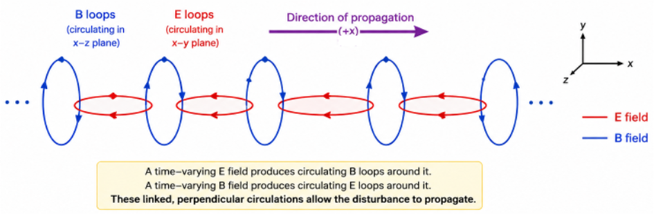
Propagation can also be illustrated using the earlier amplitude diagram, with the time axis replaced by the position () axis.

 

Previous article: Maxwell’s third equation (Faraday’s law of electromagnetic induction)

Content page of Maxwell’s equations

Content page of advanced chemistry

Main content page

Maxwell’s third equation (or Faraday’s law of electromagnetic induction) states that a time-varying magnetic field induces a circulating electric field.

This law originated from the experiments of Michael Faraday in the 1830s. As illustrated in the figure above, Faraday observed that an electromotive force (emf) is induced in a conducting loop whenever the magnetic flux through the loop changes. In one experiment, a current was produced when the loop was moved relative to a stationary magnetic field. In another, the same effect occurred when the magnetic field was moved while the loop remained fixed. Faraday also found that a current could be induced even when both the loop and the magnet were stationary, provided that the strength of the magnetic field varied with time. These observations led him to conclude that electromagnetic induction depends not on the absolute motion of the magnet or conductor, but on the rate of change of magnetic flux through the circuit. Quantitatively, the emf is proportional to the rate of change of magnetic flux,

Subsequently, Heinrich Lenz determined the direction of the induced emf. Lenz showed that the induced current always produces a magnetic field that opposes the change in magnetic flux responsible for its creation, consistent with the conservation of energy. This introduces a minus sign into Faraday’s law, giving

Here,

where is an oriented open surface bounded by the conducting loop (often visualised as a “dome” spanning the loop), is the magnetic field, and is the infinitesimal area vector associated with a surface element , with denoting the unit normal to the surface (see diagram below).

Combining eq20 and eq21 yields

To relate Faraday’s experimental law to the electric field , consider a charge moving through an infinitesimal displacement along the wire (see diagram above). The electric force acting on the charge is . Therefore, the infinitesimal work done by the electric field on the charge is

Since electric potential difference is defined as the work done per unit charge, , it follows that

The total emf around the loop is obtained by summing these infinitesimal potential differences over the entire closed path . In the limit of infinitely small segments, this becomes the line integral

Thus, the emf induced in the loop is equal to the circulation of the electric field around the closed path. Substituting this result into eq22 gives

where the time derivative may be moved inside the integral because the surface is assumed to be stationary.

This is the integral form of Maxwell’s third equation. To obtain the differential form, we apply Stokes’ theorem, which gives

Since this relation must hold for any arbitrary surface , the integrands in the second equality must be equal at every point:

This is Maxwell’s third equation in differential form. It states that a changing magnetic field generates an electric field whose field lines form closed loops around the region where the magnetic field is changing. Together with Maxwell’s fourth equation, it explains electromagnetic wave propagation.

 

 

NExt article: Maxwell’s fourth equation (corrected Ampere’s law)

Previous article: Stokes’ theorem

Content page of Maxwell’s equations

Content page of advanced chemistry

Main content page

Stokes’ theorem states that the surface integral of the curl of a vector field over an oriented surface equals the line integral of the vector field around the boundary curve of that surface.

Consider a vector field defined on an open surface  bounded by a curve (see diagram above).

Let the Cartesian axes and coincide with the edges AB and AD of an infinitesimal rectangular patch ABCD on the surface such that in the -direction, in the -direction, and . The line integral of around the boundary of ABCD is given by:

where denotes the ABCD boundary curve, the circle on the integral symbol indicates that the integration is taken over a closed curve, and .

For the edge AB, in  is constant, and so, . For the edge BC, in is a constant at , and so, . For a multivariable function , the first-order Taylor series about the point is

Evaluating at the nearby point , where gives:

Therefore,

For the edge CD, in is a constant at , and so, . Using Taylor expansion gives . Finally, for the edge DA, in is a constant at , and so, .

Summing all line integrals of the four edges yields:

Notably,

where is called the curl of .

So,

Substituting eq11 back into eq10 gives:

where .

Summing over all infinitesimal rectangle patches that partition the surface results in

where the interior edges cancel pairwise, leaving only the contribution from the outer boundary (see diagram above).

Thus, the LHS of eq13 is equivalent to the line integral of around the boundary , while the RHS becomes the surface integral of  over :

which is the mathematical expression of the Stokes’ theorem.

 

NExt article: Maxwell’s third equation (Faraday’s law of electromagnetic induction)

Previous article: Maxwell’s second equation (Gauss’ law for magnetism)

Content page of Maxwell’s equations

Content page of advanced chemistry

Main content page

Maxwell’s second equation (Gauss’s law for magnetism) states that the net magnetic flux through any closed surface is zero.

Just like the electric flux  through a surface in the derivation of Maxwell’s first equation is given by , the magnetic flux through a surface is given by:

where Gauss’s law for magnetism states that:

This law is empirical, meaning it is based on experimental observation rather than being derived from more fundamental principles. It arises from the fact that, in all experiments to date, magnetic fields have never been observed to have isolated sources or sinks (no magnetic monopoles). Instead, every magnet behaves as a dipole, with magnetic field lines forming closed loops that exit one pole and re-enter the other. This is what justifies Gauss’s law for magnetism as a fundamental postulate of classical electromagnetism.

Eq6 is the integral form of Maxwell’s second equation. Its differential form can be derived using Gauss’ theorem (also known as the divergence theorem), where . Applying the theorem to the magnetic field gives, , and hence,

For this equation to hold for any arbitrary volume , the integrand itself must be zero everywhere:

Eq7 is the differential form of Gauss’ law for magnetism.

 

NExt article: Stokes’ theorem

Previous article: Maxwell’s first equation (or Gauss’ law)

Content page of Maxwell’s equations

Content page of advanced chemistry

Main content page

Maxwell’s first equation (or Gauss’s law) states that the total electric flux through any closed surface is proportional to the electric charge enclosed within that surface.

An electric field is a vector quantity that describes the force per unit positive charge at a point in space, while the electric flux is scalar quantity that measures how much electric field passes through a surface. In other words, is obtained by integrating over a surface:

where denotes the surface integral over the closed surface , and is infinitesimal area vector normal to the surface.

Consider a sphere of radius centred on a charge . Since the electric field produced by the charge is radial and has the same magnitude at every point on the sphere, and are parallel. Therefore, .

Substituting Coulomb’s law, where into , or equivalently  since  is constant over the sphere, gives:

where the surface area of the sphere is .

Eq1 is the integral form of Maxwell’s first equation (or Gauss’s law). Although it is derived using a spherical surface, it applies to any closed surface because the electric flux through a closed surface depends only on the total charge enclosed , and not on the shape of the surface. Its differential form can be derived using Gauss’ theorem (also known as the divergence theorem) where . Applying this theorem to the electric field gives,

Since the enclosed charge can be written as , where is the charge density,

For eq2 to hold for any arbitrary volume , the underlying functions (the integrands) must be identical at every point:

which is the differential form of Gauss’ law.

The significance of Gauss’ law is that electric charges act as sources or sinks of electric field. Positive charges produce electric field lines that diverge outwards, while negative charges produce field lines that converge inwards.

 

NExt article: Maxwell’s second equation (Gauss’ law for magnetism)

Previous article: Divergence theorem (Gauss’ theorem)

Content page of Maxwell’s equations

Content page of advanced chemistry

Main content page

The divergence theorem states that the total outward flux of a vector field through a closed surface equals the integral of the field’s divergence throughout the volume enclosed by that surface.

Flux measures how much of a vector field actually passes through a surface, and only the component of the field normal to the surface contributes to the flux. This can be visualised by comparing the number of uniform field lines passing through three surfaces, each of area (see diagram above). A surface perpendicular to the field presents its full area to the flow, so the maximum number of field lines passes through it.

To compare the field lines passing through a tilted surface meaningfully, we project the surface onto a plane perpendicular to the field, which gives a reduced effective area for the flux. If we let be the angle between the field and the surface’s normal, then the projected area is . Consequently, the flux through the surface is , where is the flux density (also known as field strength), and is the area vector, with being the unit vector normal to the surface. Equivalently, , where is the component of the field normal to the surface. Therefore, only the component of the field normal to the surface contributes to the flux.

Comparatively, when the surface is parallel to the field, , resulting in a projected area of zero. No field lines pass through the surface, and the flux is zero.

To derive the mathematical expression of the divergence theorem, consider a tiny rectangular box with dimensions , and  in a vector field , where the field lines can be passing through each face of the box in any direction (see diagram below).

The flux perpendicularly through the right face of area at is

while the flux perpendicularly through the left face at is

Therefore, the net flux through the box in the -direction is:

For a multivariable function , the first-order Taylor series about the point is

Evaluating at the nearby point , where gives:

It follows that . Similarly, and . Therefore, the net total flux flowing through the box is:

where and .

Summing over yields:

where the triple integral symbol corresponds to integration with respect to the three variables , and the subscript is included for clarity to denote integration over the enclosed volume .

Now, consider a finite volume partitioned into many tiny rectangular boxes, with each interior face shared by two adjacent boxes (see diagram above). The outward flux through a shared face of one box is equal in magnitude and opposite in sign to the flux through the same face as part of the neighbouring box. As a result, all interior contributions cancel pairwise, leaving only the flux through the outer boundary surface. This converts the volume integral into a surface integral, giving the divergence theorem:

where the double integral symbol denotes integration with respect to the two variables defining a surface, and the circle on the integral symbol indicates that the integration is performed over the closed surface that bounds the volume .

 

 

Finally, the theorem is called the divergence theorem because measures the net rate at which a vector field “spreads out” (diverges) from a point. This is best illustrated using a two-dimensional diagrammatic representation of the vector field function (see diagram above), in which each point in the two-dimensional space is associated with a vector . In the first quadrant where and , the vector points up and to the right. As increases, the horizontal component increases, and as increases, the vertical component increases. Consequently, the vectors become larger and the field spreads outwards from the origin. A similar outward-spreading behaviour occurs in the other three quadrants, where the vectors also increase in magnitude as we move away from the origin. The divergence of this field is , which is constant throughout the plane. In general,

• • If , the field behaves locally like a source, with a net outward flow (positive divergence).
  • If , the point behaves locally like a sink, with a net inward flow (negative divergence). An example of such a vector field function is .
  • If , there is no net outward or inward flow (zero divergence). An example of such a vector field function is .

 

NExt article: Maxwell’s first equation (or Gauss’ law)

Content page of Maxwell’s equations

Content page of advanced chemistry

Main content page

The magnetic properties of a solid arise primarily from the spin magnetic moments of electrons and the quantum-mechanical interactions that govern their ordering within the material.

In classical electrodynamics, the relation between the magnetic dipole moment and the angular momentum is given by (see this article for derivation):

where is the classical gyromagnetic ratio.

When transitioning from classical electrodynamics to quantum mechanics, these physical observables are represented by operators: . It follows that the magnitude of an atom’s magnetic moment depends on . Consequently, even though protons and neutrons possess spin angular momentum, their contributions to the magnetic moment are much smaller than those of electrons because .

 

 

According to the Pauli Exclusion Principle, two electrons occupying the same atomic orbital have opposite spins, and therefore opposite spin magnetic moments. This is why isolated atoms with one or more unpaired electrons, such as Ag and Fe, have a net magnetic moment and are deflected in an external magnetic field.

In a solid, the situation is more complicated because atoms are no longer isolated. Instead, their outer electrons are influenced by neighbouring atoms, and the atomic orbitals broaden into energy bands, with electrons becoming delocalised throughout the crystal. Even when individual atoms carry magnetic moments, these moments do not automatically align throughout the material because the formation of magnetic order is governed by a competition between different energy contributions, in particular exchange interactions and magnetostatic energy.

The exchange interaction (also known as exchange force) is a purely quantum-mechanical effect arising from the combination of the Pauli exclusion principle and electron–electron Coulomb repulsion. As shown in a previous article, the total energy of a two-electron state depends on the symmetry of the spatial wavefunction. Due to exchange effects arising from the Pauli exclusion principle, states with parallel spins (antisymmetric spatial wavefunction) can have lower energy than those with antiparallel spins (symmetric spatial wavefunction), making the parallel configuration more stable in cases where the exchange interaction is positive. However, if a large region of the material were uniformly magnetised, it would produce a strong external stray magnetic field. This field is energetically costly because it contributes magnetostatic (demagnetising) energy.

To minimise the total energy, the material breaks up into microscopic regions called magnetic domains during formation (see diagram above). Within each domain, exchange interactions favour a roughly uniform spin alignment. Across the material, however, different domains may point in different directions, reducing the net external field and thereby lowering the magnetostatic energy. Furthermore, spins are not perfectly rigidly aligned within a domain, and small deviations can occur due to thermal fluctuations. When an external magnetic field is applied, domain walls can move so that domains aligned with the field grow at the expense of others, producing a net magnetisation of the material.

The measure of how strongly a material becomes magnetised in response to an external magnetic field strength is called the magnetic susceptibility of the material. Mathematically,

where the magnetisation is the magnetic moment per unit volume of the material.

In general, the magnetic behaviour of solids depends on how how electron spins respond to exchange interactions and external fields:

• • Ferromagnetism: In materials such as Fe, Co and Ni, exchange interactions favour parallel alignment. Domain walls can move or domains can rotate under an external field, leading to strong magnetisation. In many ferromagnets, the magnetisation is hysteretic, meaning it depends on the history of the applied field: even after the external field is removed, a residual magnetisation (remanence) can remain (see diagram below). Ferromagnets also lose their permanent magnetic properties above certain temperatures (Curie temperature or Curie point) and become paramagnetic because the higher thermal energy causes greater atomic vibrations, disrupting spin alignments. For example, Fe has a Curie temperature of approximately 770°C. Below this temperature, Fe is ferromagnetic and can be permanently magnetised. Above it, Fe becomes paramagnetic and only exhibits weak magnetism in the presence of an external magnetic field.

• • Antiferromagnetism: In materials such as MnO and NiO, the atoms are arranged with the oxide ion positioned between two metal ions, forming an M²⁺–O²⁻–M²⁺ linkage. The oxygen 2p orbital oriented along the M²⁺–O²⁻–M²⁺ bond axis contains a pair of electrons that are antiparallel, as required by the Pauli exclusion principle. One electron in this bridging orbital interacts with the metal ion on the left, while the other interacts with the metal ion on the right. Because the electron pair occupying this specific oxygen orbital is initially antiparallel, the exchange interactions mediated through the oxygen ion favour an antiparallel alignment of the neighbouring metal-ion spins, with zero net magnetisation in the absence of an external magnetic field. However, the system can still respond weakly to external fields due to thermal fluctuations.

• • Ferrimagnetism: In materials such as Fe₃O₄ (magnetite), the spins of neighbouring Fe ions are aligned antiparallel, as in antiferromagnets, but the opposing magnetic moments are unequal. This is because Fe₃O₄ can be represented as Fe³⁺[Fe²⁺Fe³⁺]O₄, with Fe³⁺ occupying tetrahedral holes and both Fe³⁺ and Fe²⁺ occupying octahedral holes (see diagram above). Because Fe³⁺ and Fe²⁺ ions are present in a 2:1 ratio, the magnetic moments of the Fe³⁺ ions largely cancel one another, leaving an uncompensated magnetic moment arising from the Fe²⁺ ions. As a result, the material possesses a non-zero net magnetisation and exhibits domain behaviour and hysteresis similar to those of ferromagnets. In fact, the strongest permanent magnets, such as neodymium magnets, exhibit ferrimagnetism.

• • Paramagnetism: In materials such as Al and Pt (including O₂ gas), atomic magnetic moments are largely independent in the absence of strong exchange interactions. They align weakly and only temporarily with an applied magnetic field due to thermal agitation, and the magnetisation disappears when the field is removed.

• • Diamagnetism: In materials such as Cu, Ag and Au (including H₂O), there are no permanent magnetic moments from unpaired electrons. An applied magnetic field induces small circulating currents that oppose the applied field, producing a weak, negative magnetisation that is present only while the field is applied. In fact, all materials exhibit diamagnetism to some extent due to Lenz’ law. In paramagnetic and ferromagnetic materials, however, this effect is usually overwhelmed by stronger magnetic mechanisms. Because diamagnetic materials are repelled by magnetic fields, they can be levitated in sufficiently strong magnetic field gradients. A notable example is the levitation of superconductors, which behave as perfect diamagnets due to the Meissner effect.

 

 

Ultimately, a solid’s magnetic identity is not a static property, but a dynamic equilibrium dictated by this delicate balance between quantum-scale spin ordering and large-scale thermodynamic and electrostatic forces.

 

 

 

NExt article: Neodymium Magnets

Previous article: Superconductor

Content page of solid-state chemistry

Content page of advanced chemistry

Main content page

Neodymium magnets are permanent magnets made primarily from an alloy of neodymium, iron and boron (NdFeB), and are the strongest commercially available type of permanent magnet.

Pure iron is strongly ferromagnetic because of exchange interactions among its 3d electrons. However, despite its large magnetisation, it is not an ideal permanent magnet because its magnetic domains can reorient relatively easily in response to external magnetic fields, reflecting its weak magnetocrystalline anisotropy.

When iron is alloyed with rare-earth elements such as neodymium, additional exchange interactions arise between the rare-earth and iron atoms. Although the 4f orbitals of rare-earth elements are partially filled and carry substantial magnetic moments, they are spatially compact and lie deep within the atom. Consequently, the 4f electrons are highly localised and do not interact directly with the 3d electrons of iron. Instead, the coupling occurs through an indirect exchange mechanism involving the rare-earth 5d electrons.

This mechanism is a two-step coupling process. While the 5d shell of an isolated rare-earth atom is empty in its ground state, the formation of a metallic crystal lowers the energy of the 5d-derived states through bonding interactions, allowing some valence electrons to occupy them. In the first step, the localised 4f electrons interact through strong intra-atomic exchange with these more spatially extended 5d electrons, causing the spins of the 4f and 5d electrons to align (see diagram below).

In the second step, the diffuse rare-earth 5d orbitals overlap with the 3d orbitals of neighbouring iron atoms, lowering the total energy of the crystal. This resulting exchange interaction is governed by the Pauli exclusion principle, which restricts how electrons of the same spin can occupy overlapping states. The lowest-energy configuration generally corresponds to antiparallel alignment between the rare-earth 5d spin and the iron 3d spin. Since the rare-earth 4f and 5d spins are already aligned from the first step, it follows that the rare-earth 4f spin and the iron 3d spin tend to align antiparallel. In this way, the localised 4f moments of the rare-earth ions become indirectly coupled to the iron sublattice.

However, because the total magnetic moment of a rare-earth ion is contingent on both spin and orbital angular momentum, the resulting alignment of the rare-earth magnetic moment relative to iron depends on Hund’s rules.

Consider the following rare-earth electron configurations, noting that the 4f subshell can accommodate up to 14 electrons:

Nd: [Xe]4f⁴6s² (less than half-filled 4f subshell)

Tb: [Xe]4f⁹6s² (more than half-filled 4f subshell)

Dy: [Xe]4f¹⁰6s² (more than half-filled 4f subshell)

According to Hund’s third rule, the ground state of Nd is characterised by J = L − S, whereas those of Tb and Dy are characterised by J = L + S. Consequently, the total Nd magnetic moment is oriented opposite to its spin angular momentum, while the Tb and Dy total magnetic moments are aligned with their spins. Since the Nd 4f spin is coupled antiparallel to the Fe 3d spin through indirect exchange mediated by the rare-earth 5d states, the total magnetic moment of Nd aligns parallel to that of iron, resulting in ferrimagnetic alignment between the Nd and Fe sublattices. In contrast, the total magnetic moments of Tb and Dy align antiparallel to the magnetic moment of iron, producing ferrimagnetic ordering in Tb–Fe and Dy–Fe systems with a reduced net magnetic moment.

Nevertheless, Nd and Fe alone do not readily form a stable crystal structure. This issue is resolved by adding boron to produce the inter-metallic compound Nd₂Fe₁₄B. In this phase, boron plays a crucial structural role in stabilising a complex tetragonal lattice that accommodates both a high density of Fe atoms and well-ordered Nd sites, resulting in a crystal with strong exchange-driven magnetisation and large magnetocrystalline anisotropy.

In practice, neodymium magnets are engineered so that the Nd₂Fe₁₄B phase constitutes the majority of the material. The remaining volume (10–15%) consists primarily of Nd-rich grain-boundary phases that separate neighbouring magnetic grains (see diagram above). If neighbouring Nd₂Fe₁₄B grains were strongly exchange-coupled throughout the entire magnet, reversal of the magnetic moment in one grain could more easily propagate into adjacent grains, reducing coercivity (i.e. the resistance to demagnetisation). By partially isolating neighbouring grains, the Nd-rich boundary phase inhibits the propagation of reversed magnetic domains and significantly improves coercivity.

Neodymium magnets are typically manufactured using a powder-metallurgy process. An alloy containing neodymium, iron and boron is first melted and cast, then crushed into a fine powder. The powder particles are aligned in a strong magnetic field so that their crystallographic-easy axes point in the same direction, maximising the magnetic performance of the final magnet. The aligned powder is then compacted and sintered at high temperature to form a dense solid. Subsequent heat-treatment steps optimise the microstructure by promoting the formation of Nd-rich grain-boundary phases that enhance coercivity. In addition, small amounts of Dy and Tb are often incorporated into the alloy to further increase coercivity and improve magnetic stability at elevated operating temperatures. Finally, the magnet is machined to the required shape, coated to improve corrosion resistance, and magnetised using a strong external magnetic field.

Applications that require strong magnetic fields in a compact volume often rely on neodymium magnets. Examples include electric vehicle traction motors, wind turbine generators, computer hard disk drives, magnetic resonance imaging (MRI) systems, industrial actuators, and consumer electronics such as headphones, loudspeakers and smartphones.

Previous article: Magnetic properties of a solid

Content page of advanced chemistry

Main content page