The Bose–Einstein distribution describes how indistinguishable bosons are distributed among available energy states at thermal equilibrium.
To derive the Bose–Einstein distribution, consider a system of fixed-volume containing bosons occupying discrete single-particle energy levels
, each with degeneracy
, with no restriction on the number of bosons that can occupy a single state. The total number of bosons
and the total energy
of the system are
where
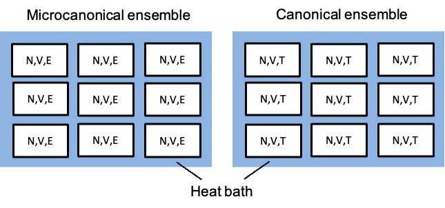
Replicas of this system form a microcanonical ensemble, meaning that only configurations with the same fixed
and
are allowed.
Since any number of bosons can occupy the same single-particle state, the number of ways to place
bosons among the
degenerate states at energy
is given by the stars-and-bars result:
For example, if two bosons occupy three degenerate states (
), the possible occupation configurations are 200, 020, 002, 110, 101, or 011. Thus, there are six possible microstates, consistent with
It follows that the total number of microstates corresponding to a particular configuration is
For macroscopic systems, distinct single-particle energy levels are often extremely closely spaced. Consequently, many distinct energy levels can fall within a small energy interval. For the purposes of counting, these closely spaced levels may be treated as approximately degenerate, so that the interval contains a very large number of approximately degenerate single-particle states. Taking the natural logarithm of eq34 and substituting eq33 gives:
where because
is large.
Using Stirling’s approximation. where , yields:
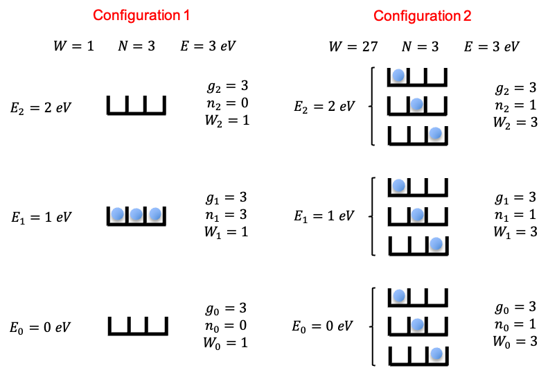
The possible configurations that define the microcanonical ensemble are restricted by eq31 and eq32. For example, the configurations and
generally have different total energies and therefore cannot both belong to the same microcanonical ensemble. However, different configurations can have the same total energy and therefore can belong to the same microcanonical ensemble (see above diagram for an illustration). In such cases, all microstates corresponding to the allowed configurations satisfying the fixed
and
constraints are equally probable. The most probable equilibrium configuration is therefore the one with the largest number of ways of achieving it, i.e. the one whose
(or
) is maximal.
The total differential of is:
Hence, we want to solve for . With reference to Step 2 of the derivation of the Boltzmann distribution using the Lagrange method of undetermined multipliers, eq36 becomes:
where we have chosen minus signs for the 2nd and 3rd terms for convenience.
Since varies independently, eq37 holds only if each coefficient is zero:
Substituting eq35 into eq38, and noting that does not depend on
, gives:
where we have changed the summation index from to
in eq39 to distinguish the summation variable from the differentiation variable.
All terms in the summation of eq39 goes to zero except when . So,
Carrying out the differentiation and rearranging the result yields:
As mentioned above, is the number of bosons occupying the energy level
. To transform eq40 into a probability distribution, we write:
where is the average or expected occupation number per degenerate state at energy
. Thus,
gives the total number of bosons occupying
.
Substituting eq41 into eq40 gives:
The evaluation of the Lagrange multipliers and
proceeds in exactly the same way as for the Fermi-Dirac distribution, resulting in
and
. Therefore,
which is the Bose–Einstein distribution function.
For bosons, the chemical potential must satisfy
, where
is the lowest single-particle energy level. This condition ensures that the denominator in eq43 does not become negative or zero. In particular, when the ground-state energy is chosen to be zero (
), the chemical potential satisfies
. As
approaches the ground-state energy from below (
), the occupation of the lowest-energy state can become extremely large because
This behaviour is associated with Bose–Einstein condensation, in which a macroscopic number of bosons can occupy the lowest-energy quantum state.
For photons , the situation is slightly different. Although photons are bosons, their number is not conserved in thermal equilibrium because they can be freely created and absorbed through interactions with matter, e.g.
. The chemical potential of a species is defined as the change in Gibbs free energy
with respect to the change in the number of particles of that species
, while the temperature, pressure and numbers of all other species are held constant:
. Since
is a minimum at equilibrium,
if
is free to vary. If
is constrained and not free to vary, then
may or may not be zero. Consequently, the chemical potential of photons is always zero at thermodynamic equilibrium, and eq43 becomes
which is the occupation factor underlying Planck’s blackbody radiation law, showing that blackbody radiation is fundamentally a quantum-statistical phenomenon.