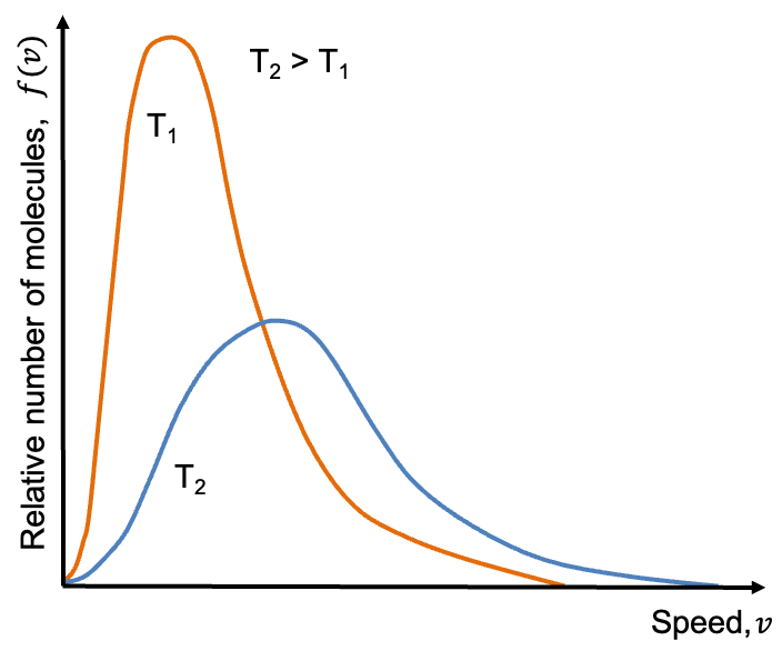
The Maxwell-Boltzmann distribution \(f(v)\) describes the range of speeds \(v\) among gaseous molecules of an ideal gas at a given temperature \(T\).
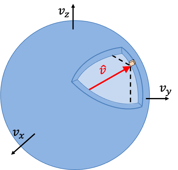
The energy of an ideal gas molecule of mass \(m\) is characterised solely by its kinetic energy \(E\). For a molecule with velocity \(\hat{v}\), its energy is \(\small{E=\frac{1}{2}mv_x^2+\frac{1}{2}mv_y^2+\frac{1}{2}mv_z^2}\), where \(\small{v_x}\), \(\small{v_y}\) and \(\small{v_z}\) are the velocity vector components of \(\hat{v}\) in Cartesian coordinates. Given that a molecule with the velocity magnitude \(\small{\vert\hat{v}_i\vert=v_i}\) has the same energy regardless of direction, any molecule with the ordered triple \(\small{(v_x,v_y,v_z)}\) that lies on the surface of a sphere of radius \(\small{v_i}\) in velocity space belongs to the energy state \(\small{\varepsilon_i=\frac{1}{2}mv_{x,i}^2+\frac{1}{2}mv_{y,i}^2+\frac{1}{2}mv_{,i}z^2}\) (see diagram below).

The fraction of molecules in the energy state \(\small{\varepsilon_i}\) is given by the Boltzmann distribution:
$$\frac{n_i}{N}=\frac{e^{-\frac{\varepsilon_i}{kT}}}{\sum_ie^{-\frac{\varepsilon_i}{kT}}}\;\;\;\;\;\;\;\;1$$
where
\(k\) is the Boltzmann constant.
\(T\) is the equilibrium temperature of the system.
\(\small{n_i}\) is the number of molecules in the energy state.
\(N\) is the total number of molecules in the system.
In probability theory, \(\small{\frac{n_i}{N}}\) is the probability \(\small{p_i}\) of molecules in state \(i\), with \(\small{\sum_ie^{-\frac{\varepsilon_i}{kT}}}\) being the normalisation constant. In other words, \(\small{p_i\propto e^{-\frac{\varepsilon_i}{kT}}}\), which we can rewrite as:
$$f(v_x,v_y,v_z)=Ke^{-\frac{m(v_x^2+v_y^2+v_z^2)}{2kT}}\;\;\;\;\;\;\;\;2$$
where \(\small{f(v_x,v_y,v_z)}\) is the probability density function (probability per unit interval of \(v\) ) of molecules in a particular energy state \(\small{\frac{1}{2}mv_x^2+\frac{1}{2}mv_y^2+\frac{1}{2}mv_z^2}\) (we have dropped the index \(i\) for convenience) and \(K\) is the proportionality constant.
Since \(\small{f(v_x,v_y,v_z)=\biggr(K^{\prime}e^{-\frac{mv_x^2}{2kT}}\biggr)\biggr(K^{\prime}e^{-\frac{mv_y^2}{2kT}}\biggr)\biggr(K^{\prime}e^{-\frac{mv_z^2}{2kT}}\biggr)=f(v_x)f(v_y)f(v_z)}\), where \(\small{K^{\prime}=K^{1/3}}\),
$$f(v_x,v_y,v_z)=Ke^{-\frac{mv_x^2}{2kT}}e^{-\frac{mv_y^2}{2kT}}e^{-\frac{mv_z^2}{2kT}}\;\;\;\;\;\;\;\;3$$
As the probability density function \(\small{f(v_x,v_y,v_z)}\) is separable, its normalisation is equivalent to the separate normalisation of each of the individual functions:
$$\int_{-\infty}^{\infty}f(v_x)dv_x=1\;\;\;\;\int_{-\infty}^{\infty}f(v_y)dv_y=1\;\;\;\;\int_{-\infty}^{\infty}f(v_z)dv_z=1\;\;\;\;\;\;\;\;4$$
Let’s evaluate just one of the integrals in eq4 by substituting \(\small{f(v_x)=K^{1/3}e^{-\frac{mv_x^2}{2kT}}}\) in \(\small{\int_{-\infty}^{\infty}f(v_x)dv_x=1}\) to give
$$K^{\frac{1}{3}}\int_{-\infty}^{\infty}e^{-\frac{mv_x^2}{2kT}}dv_x=1\;\;\;\;\;\;\;\;5$$

Question
Show that \(\small{\int_{-\infty}^{\infty}e^{-aX^2}dX=\sqrt{\frac{\pi}{a}}}\).
Answer
Let \(\small{I=\int_{-\infty}^{\infty}e^{-aX^2}dX}\) and at the same time let \(\small{I=\int_{-\infty}^{\infty}e^{-aY^2}dY}\) since \(X\) and \(Y\) are dummy variables.
$$I^2=\int\int_{-\infty}^{\infty}e^{-a(X^2+Y^2)}dXdY$$
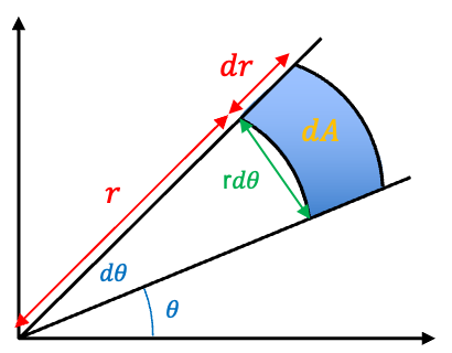
In polar coordinates, \(r^2=X^2+Y^2,X=rcos\theta,Y=rsin\theta\). For infinitesimal changes, the change in area \(dA\) can be approximated as a rectangle with sides \(r\) and \(rd\theta\) (see diagram below), with \(dXdY=dA=rd\theta dr\).
So,
$$I^2=\int_{0}^{2\pi}d\theta\int_{0}^{\infty}re^{-r^2}dr=2\pi\int_{0}^{\infty}re^{-r^2}dr$$
Let \(u=r^2\;\Rightarrow\;du=2rdr\)
$$I^2=2\pi\int_{0}^{\infty}re^{-au}\frac{du}{2r}=\pi\int_{0}^{\infty}e^{-au}du=\frac{\pi}{a}\;\;\Rightarrow\;\;I=\sqrt{\frac{\pi}{a}}$$
Hence, eq5 becomes,
$$K=\biggr(\frac{m}{2\pi kT}\biggr)^{\frac{3}{2}}\;\;\;\;\;\;\;\;6$$
Substituting eq6 in eq3,
$$f(v_x,v_y,v_z)=\biggr(\frac{m}{2\pi kT}\biggr)^{\frac{3}{2}}e^{-\frac{mv_x^2}{2kT}}e^{-\frac{mv_y^2}{2kT}}e^{-\frac{mv_z^2}{2kT}}\;\;\;\;\;\;\;\;7$$
Eq7 is known as the Maxwell-Boltzmann distribution for the velocity vector of a molecule. The fraction of molecules \(\small{dn_{v_xv_yv_z}/N}\) with velocity vectors in the infinitesimal range of \(\small{v_x}\) to \(\small{v_x+dv_x}\), \(\small{v_y}\) to \(\small{v_y+dv_y}\) and \(\small{v_z}\) to \(\small{v_z+dv_z}\) is
$$\frac{dn_{v_xv_yv_z}}{N}=f(v_x,v_y,v_z)dv_xdv_ydv_z=\biggr(\frac{m}{2\pi kT}\biggr)^{\frac{3}{2}}e^{-\frac{m(v_x^2+v_y^2+v_z^2)}{2kT}}dv_xdv_ydv_z\;\;\;\;\;\;\;\;8$$
The fraction of molecules \(\small{dn_v/N}\) with speed in the infinitesimal range of \(v\) to \(v+dv\) is then equivalent to the fraction of molecules with velocity vectors that lies within a spherical shell of infinitesimal thickness in velocity space (see diagram below).
In other words,
$$\frac{dn_v}{N}=\biggr(\frac{m}{2\pi kT}\biggr)^{\frac{3}{2}}e^{-\frac{mv^2}{2kT}}\sum_{shell}dv_xdv_ydv_z$$
where \(\small{v^2=v_x^2+v_y^2+v_z^2}\), and we have assumed that the volume of the shell of infinitesimal thickness is approximately equal to the sum of infinitesimal cubes, each with an infinitesimal volume of \(\small{dv_xdv_ydv_z}\).
Therefore, \(\small{\sum_{shell}dv_xdv_ydv_z=4\pi v^2dv}\) and \(\small{\frac{dn_v}{N}=f(v)dv=4\pi\biggr(\frac{m}{2\pi kT}\biggr)^{\frac{3}{2}}v^2e^{-\frac{mv^2}{2kT}}dv}\)., which implies that the probability density function for the speed of a molecule \(f(v)\) is
$$f(v)=4\pi\biggr(\frac{m}{2\pi kT}\biggr)^{\frac{3}{2}}v^2e^{-\frac{mv^2}{2kT}}\;\;\;\;\;\;\;\;9$$
Eq9 is known as the Maxwell-Boltzmann distribution for the speed of a molecule. It also expresses the probability of a molecule being associated with a particular energy state. For a mole of an ideal gas, we substitute \(R=N_Ak\) (see this article for derivation ) in eq9 to give
$$f(v)=4\pi\biggr(\frac{M}{2\pi RT}\biggr)^{\frac{3}{2}}v^2e^{-\frac{Mv^2}{2RT}}\;\;\;\;\;\;\;\;10$$
where \(M\) is the mass of one mole of the gas and \(R\) is the gas constant.
Question
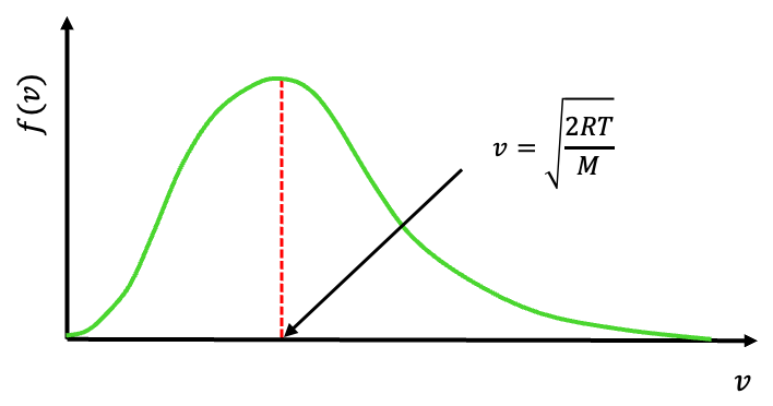
Show that the most probable speed of one mole of an ideal gas is \(\small{v=\sqrt{\frac{2RT}{M}}}\).
Answer
The most probable speed corresponds to the peak of the distribution (see above diagram). Carrying out the derivative \(\small{\frac{df(v)}{dv}}\) , equating it to zero, and noting that the most probable speed \(v\) is neither \(0\) nor \(\infty\), we have \(\small{v=\sqrt{\frac{2RT}{M}}}\).