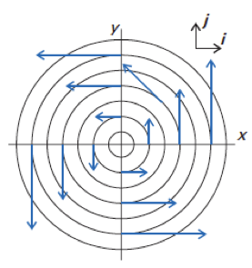
In classical electrodynamics, a magnetic dipole moment  is associated with a current loop (see diagram below), and represents the magnitude and orientation of a magnetic dipole. It is a pseudo-vector, whose direction is perpendicular to the plane of the loop and given by the right hand thumb rule.
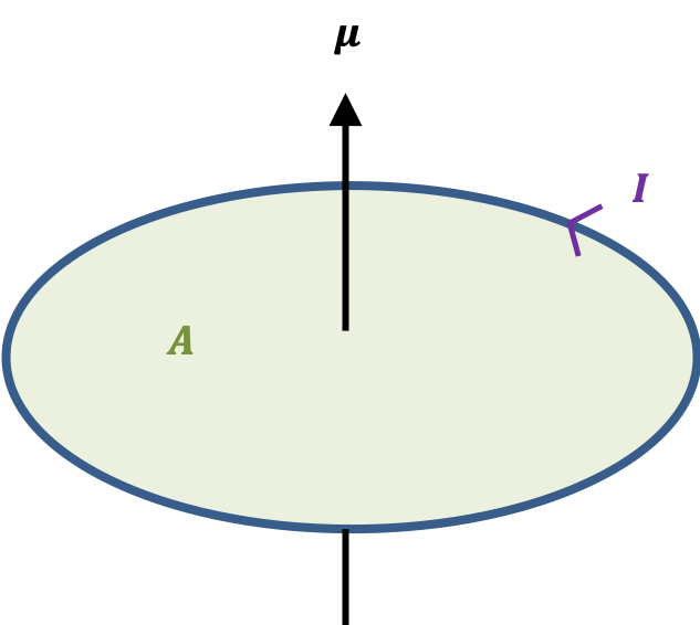
The magnitude of a magnetic dipole moment of a current loop is defined as

where  is current, and
  is the area of the loop.
Rewriting eq60 in terms of  (where
  is charge,
  is time and
  is the tangential velocity of the charged particle) and using
  , we have
  , where
  is the mass of the charged particle. Substitute eq59 in , we have the relation between magnetic dipole moment and angular momentum:

where  is the classical gyromagnetic ratio.
When placed in an external magnetic field , the magnetic dipole moment experiences a torque, whose energy is


Question
How is eq62 derived?
Answer
In order to rotate a current loop, we must do work  against the torque
  due to the magnetic field
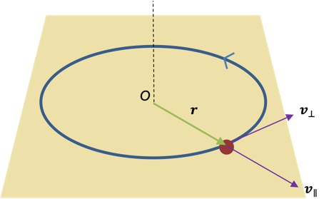
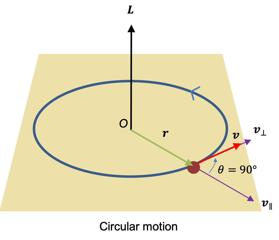
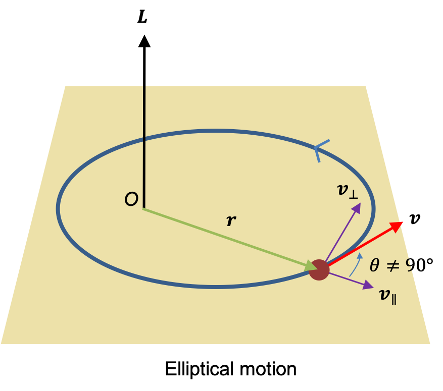
  . For a rotating system (see diagram I below),
  , where according to convention, the negative sign is added so that work on the system by the field is positive.
For small  ,
,  . Since
  and
and  , we have

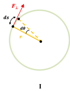
Diagram II below shows a square current loop with side 1 parallel to side 3 and side 2 parallel to side 4 (not shown in diagram). The length of each side is  .
.
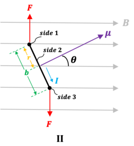
Since  and
and  (
( ),
),
\;&space;\;&space;\;&space;\;&space;\;&space;\;&space;\;&space;\;&space;62b)
where is the area of the loop.
Substitute eq60 in the above equation,
\;&space;\;&space;\;&space;\;&space;\;&space;\;&space;\;&space;\;&space;63)
Comparing eq62a and eq62b, torque can also be expressed as

The torque exerted by the magnetic field on the magnetic dipole tends to rotate the dipole towards a lower energy state. So, we let  with
with  and eq63 becomes
  , or simply:

Other than a torque, the external magnetic field may exert another force on the current loop. For a magnetic field pointing in the  -direction,
 \boldsymbol{\mathit{k}}) , where
, where ) is a scalar function. We substitute eq65 in
is a scalar function. We substitute eq65 in  to give
![\boldsymbol{\mathit{F_z}}=\frac{\partial(\boldsymbol{\mathit{\mu}}\cdot\boldsymbol{\mathit{B}})}{\partial z}=\frac{\partial[(\mu_x\boldsymbol{\mathit{i}}+\mu_y\boldsymbol{\mathit{j}}+\mu_z\boldsymbol{\mathit{k}})\cdot B_z(x,y,z)\boldsymbol{\mathit{k}}]}{\partial z}=\mu_z\frac{\partial B_z(x,y,z)}{\partial z}\; \; \; \; \; \; \; \; 66](https://latex.codecogs.com/gif.latex?\boldsymbol{\mathit{F_z}}=\frac{\partial(\boldsymbol{\mathit{\mu}}\cdot\boldsymbol{\mathit{B}})}{\partial&space;z}=\frac{\partial[(\mu_x\boldsymbol{\mathit{i}}+\mu_y\boldsymbol{\mathit{j}}+\mu_z\boldsymbol{\mathit{k}})\cdot&space;B_z(x,y,z)\boldsymbol{\mathit{k}}]}{\partial&space;z}=\mu_z\frac{\partial&space;B_z(x,y,z)}{\partial&space;z}\;&space;\;&space;\;&space;\;&space;\;&space;\;&space;\;&space;\;&space;66)
where  ,
,  and
and  are unit vectors, and
 }{\partial&space;z}) is the gradient of the external magnetic field along the -direction.
is the gradient of the external magnetic field along the -direction.
For a uniform field, =B_0) (i.e. a constant) and
(i.e. a constant) and  ; while for an inhomogenous field,
 =B_0+\alpha&space;z) , where
, where  is a scalar representing the change in
  along the -axis, and
  .
.
Substituting eq61 in eq62,

For an inhomogenous magnetic field pointing in the -direction, the above equation becomes
\boldsymbol{\mathit{k}}\cdot(L_x\boldsymbol{\mathit{i}}+L_y\boldsymbol{\mathit{j}}+L_z\boldsymbol{\mathit{k}})=-\gamma(B_0+\alpha&space;z)L_z\;&space;\;&space;\;&space;\;&space;\;&space;\;&space;\;&space;\;&space;68)
Eq68 is used as a starting point in analysing results from the Stern-Gerlach experiment.