The Stern-Gerlach experiment, which was conducted in 1922 by Otto Stern and Walther Gerlach, showed that electrons have quantised spin angular momentum. In a typical Stern-Gerlach experiment, silver is vapourised in an oven, creating silver atoms, which after being collimated, pass through an inhomogeneous magnetic field and eventually deposit on a detector plate (see diagram below).
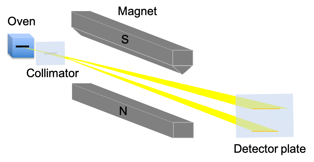
A silver atom is electrically neutral and has a single unpaired valence electron, whose orbital angular momentum is zero, as it resides in an s-orbital. The other 46 electrons occupy 4 closed shells and have zero total orbital angular momentum. These electronic properties of silver indicate that the beam of atoms will travel undeflected through the magnet. However, the beam is split symmetrically into two, with the atoms deposited on the detector plate in two horizontal lines. This propounds, according to classical physics (see eq66), that a silver atom possesses a non-zero magnetic dipole moment, which implies that the atom has some form of intrinsic angular momentum other than orbital angular momentum. Furthermore, eq66 and the symmetric splitting of the beam together suggest that there are two non-zero magnetic dipole moment involved, both of equal magnitude but in opposite directions. Therefore (with reference to eq65), a portion of the silver atoms must be in a different energy state versus the rest of the atoms.

Question
Why electrons occupying any closed shell of principal quantum number (where
) have zero total orbital angular momentum?
Answer
We know that the relation between a shell and its sub-shells
is
. We also know from eq132 that
, where
. Furthermore, every sub-shell consists of one or more orbitals, each of which can hold 2 electrons. Therefore, for any closed shell, the sum of all
is zero and so, the total orbital angular momentum is zero.
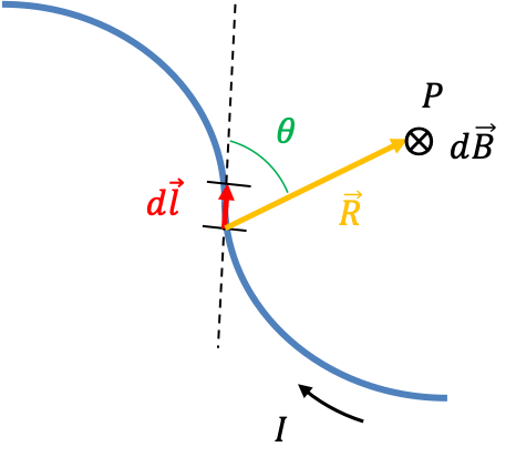
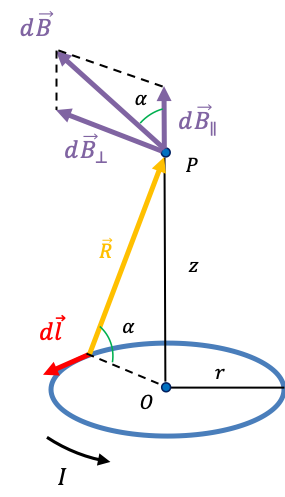
To explain the results of the experiment, we need to derive a quantum mechanical expression that allows us to analyse the energy of a silver atom passing through the inhomogenous magnetic field. A reasonable starting point is eq68:
The quantum mechanical expression of the above classical equation, which is based on the current loop model, is obtained by replacing the potential energy term and the
-component of angular momentum term
with the energy operator
(Hamiltonian) and the
-component angular momentum operator
respectively:
If we postulate that the intrinsic angular momentum operator is the analogue of
, we can rewrite the above equation as:
We have also replaced the classical gyromagnetic ratio with a factor
. The significance of this will be apparent at the end of the article. Assuming that the Hamiltonian
acts on the intrinsic angular momentum eigenvector
for a duration of
when the silver atom passes through the magnet, it needs to be represented by a time-dependent operator:
Since is the analogue of
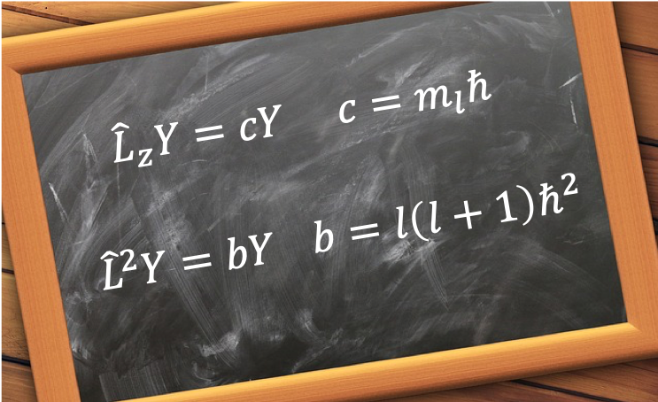
, we can also assume that the eigenvalue equations corresponding to eq132 and eq133 are:
where and
(unlike quantum numbers for orbital angular momentum, we did not restrict
and
to integers because we have no reason to do so).
As mentioned earlier, the silver atoms are split into two beams, implying two different energy states. In quantum mechanics, the state of atoms in each beam is described by a distinct set of quantum numbers. Hence, the state of atoms in one beam must be characterised by and the other by
. However, we cannot tell which atom is which prior to
. It is therefore appropriate to express the time-dependent solution to eq158 prior to
as a linear combination of the two states:
where and
are constants;
and
are the time-independent components of
and
respectively.
Since , the eigenvalues of
are
, and hence from eq158,
In summary, the 2 energy states described in eq162 are due to a silver atom’s intrinsic angular momentum, which is characterised by the quantum numbers and
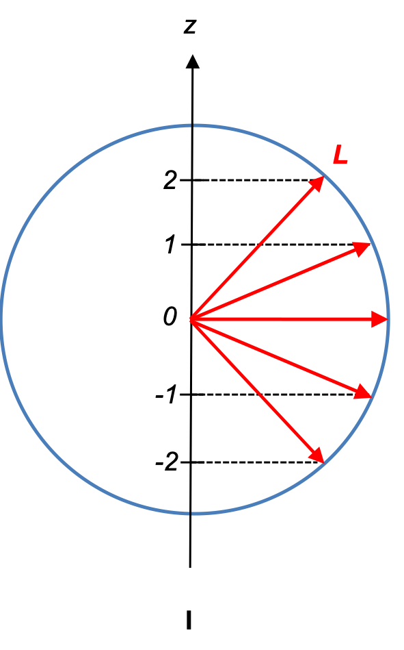
. Since, the magnetic dipole moment of a silver atom’s nucleus is very weak (see below for details), the intrinsic angular momentum is attributed to that of an electron (in this case, the single unpaired valence electron). George Uhlenbeck and Samuel Goudsmit, together with Wolfgang Pauli called it spin. The quantum number
is subsequently found in another experiment to be
, which makes
.
Question
What is the definition of and how it is different from
?
Answer
According to classical physics, we would expect to be equal to
. However, the value of
is determined in another experiment to be about twice the classical value. Due to this difference, the classical notion of the electron spinning on its own axis (which is equivalent to a current loop) has no physical reality.

Question
i) How does nuclear spin affect the experiment?
ii) Show that the change in energy of a nuclear magnetic dipole moment in the presence of a uniform magnetic field is .
Answer
i) From eq61, the magnetic dipole moment in the -direction that is due to an electron’s spin angular momentum is
. The magnetic dipole moment of an atom’s nucleus is usually due to only one nucleon (magnetic dipole moment of an atom with even-even nucleons is negligible):
Therefore, the typical nuclear magnetic dipole moment is much weaker than an electron magnetic dipole moment. A magnetic field much stronger (Stern-Gerlach experiment ) is needed to achieve reasonable resolution.
ii) The corresponding nuclear spin energy operator equation of eq68 in a uniform magnetic field is
. With reference to eq168, the eigenvalue of
is
or
, since
.
For sequential Stern-Gerlach experiments, see this article.