The magnetic properties of a solid arise primarily from the spin magnetic moments of electrons and the quantum-mechanical interactions that govern their ordering within the material.
In classical electrodynamics, the relation between the magnetic dipole moment and the angular momentum
is given by (see this article for derivation):
where is the classical gyromagnetic ratio.
When transitioning from classical electrodynamics to quantum mechanics, these physical observables are represented by operators: . It follows that the magnitude of an atom’s magnetic moment depends on
. Consequently, even though protons and neutrons possess spin angular momentum, their contributions to the magnetic moment are much smaller than those of electrons because
.

Question
Does the orbital angular momentum of an electron contribute to the magnetic moment of an atom?
Answer
Yes, it does. However, the contribution of orbital angular momentum to the magnetic moment is about half that of spin angular momentum. For an electron, the gyromagnetic ratio can be written as , where
is the
-factor. Since orbital angular momentum arises from the electron’s spatial degrees of freedom, its associated gyromagnetic ratio has the classical form, corresponding to
. In contrast, spin angular momentum is an intrinsic quantum property of the electron, with
experimentally determined to be approximately 2.
According to the Pauli Exclusion Principle, two electrons occupying the same atomic orbital have opposite spins, and therefore opposite spin magnetic moments. This is why isolated atoms with one or more unpaired electrons, such as Ag and Fe, have a net magnetic moment and are deflected in an external magnetic field.
In a solid, the situation is more complicated because atoms are no longer isolated. Instead, their outer electrons are influenced by neighbouring atoms, and the atomic orbitals broaden into energy bands, with electrons becoming delocalised throughout the crystal. Even when individual atoms carry magnetic moments, these moments do not automatically align throughout the material because the formation of magnetic order is governed by a competition between different energy contributions, in particular exchange interactions and magnetostatic energy.
The exchange interaction (also known as exchange force) is a purely quantum-mechanical effect arising from the combination of the Pauli exclusion principle and electron–electron Coulomb repulsion. As shown in a previous article, the total energy of a two-electron state depends on the symmetry of the spatial wavefunction. Due to exchange effects arising from the Pauli exclusion principle, states with parallel spins (antisymmetric spatial wavefunction) can have lower energy than those with antiparallel spins (symmetric spatial wavefunction), making the parallel configuration more stable in cases where the exchange interaction is positive. However, if a large region of the material were uniformly magnetised, it would produce a strong external stray magnetic field. This field is energetically costly because it contributes magnetostatic (demagnetising) energy.
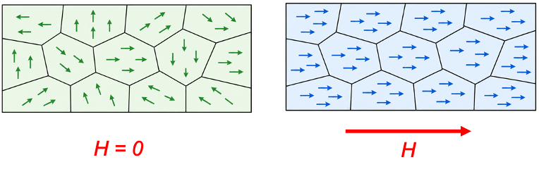
To minimise the total energy, the material breaks up into microscopic regions called magnetic domains during formation (see diagram above). Within each domain, exchange interactions favour a roughly uniform spin alignment. Across the material, however, different domains may point in different directions, reducing the net external field and thereby lowering the magnetostatic energy. Furthermore, spins are not perfectly rigidly aligned within a domain, and small deviations can occur due to thermal fluctuations. When an external magnetic field is applied, domain walls can move so that domains aligned with the field grow at the expense of others, producing a net magnetisation of the material.
The measure of how strongly a material becomes magnetised in response to an external magnetic field strength is called the magnetic susceptibility
of the material. Mathematically,
where the magnetisation is the magnetic moment per unit volume of the material.
In general, the magnetic behaviour of solids depends on how how electron spins respond to exchange interactions and external fields:
-
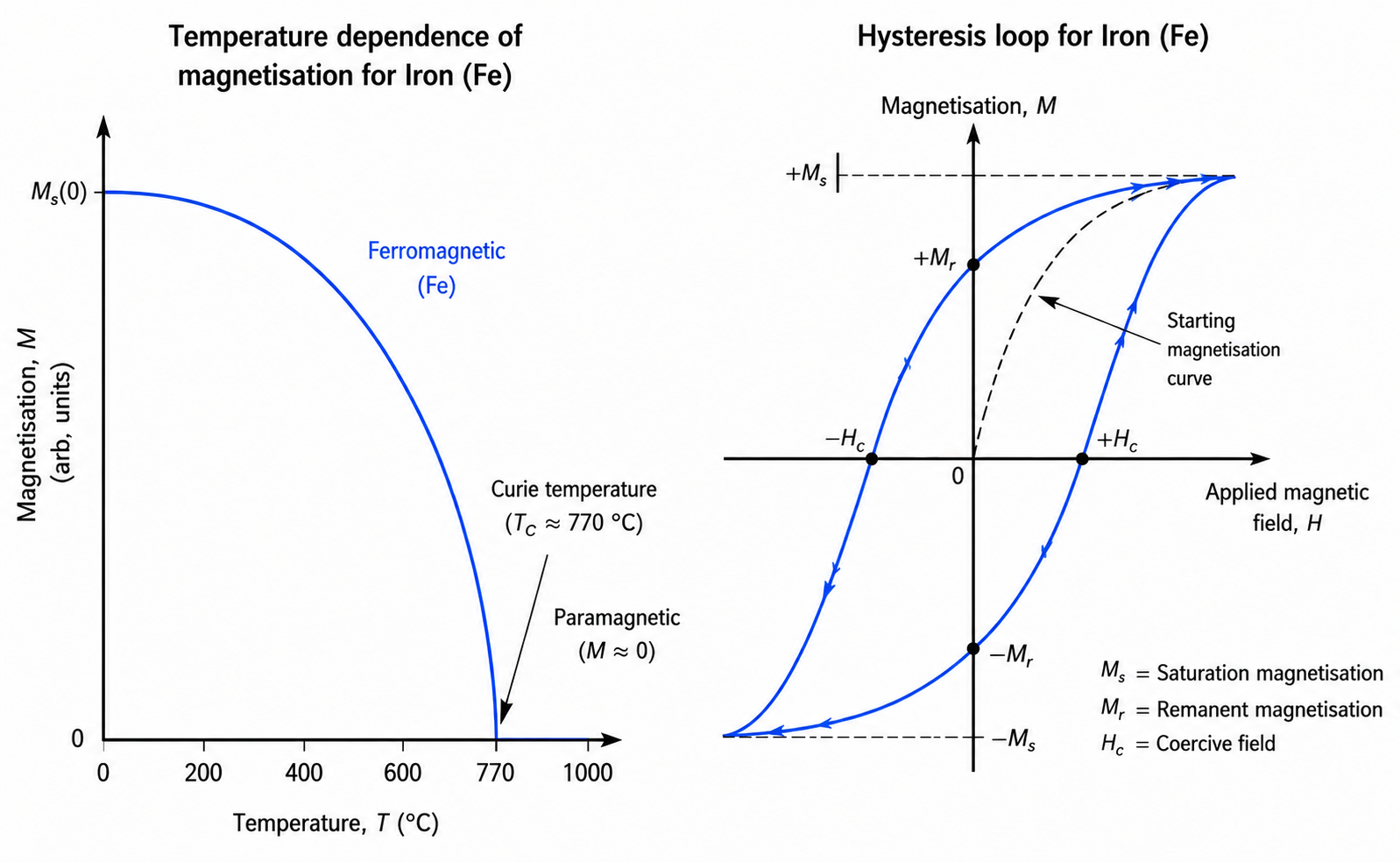
- Ferromagnetism: In materials such as Fe, Co and Ni, exchange interactions favour parallel alignment. Domain walls can move or domains can rotate under an external field, leading to strong magnetisation. In many ferromagnets, the magnetisation is hysteretic, meaning it depends on the history of the applied field: even after the external field is removed, a residual magnetisation (remanence) can remain (see diagram below). Ferromagnets also lose their permanent magnetic properties above certain temperatures (Curie temperature or Curie point) and become paramagnetic because the higher thermal energy causes greater atomic vibrations, disrupting spin alignments. For example, Fe has a Curie temperature of approximately 770°C. Below this temperature, Fe is ferromagnetic and can be permanently magnetised. Above it, Fe becomes paramagnetic and only exhibits weak magnetism in the presence of an external magnetic field.
-
- Antiferromagnetism: In materials such as MnO and NiO, the atoms are arranged with the oxide ion positioned between two metal ions, forming an M²⁺–O²⁻–M²⁺ linkage. The oxygen 2p orbital oriented along the M²⁺–O²⁻–M²⁺ bond axis contains a pair of electrons that are antiparallel, as required by the Pauli exclusion principle. One electron in this bridging orbital interacts with the metal ion on the left, while the other interacts with the metal ion on the right. Because the electron pair occupying this specific oxygen orbital is initially antiparallel, the exchange interactions mediated through the oxygen ion favour an antiparallel alignment of the neighbouring metal-ion spins, with zero net magnetisation in the absence of an external magnetic field. However, the system can still respond weakly to external fields due to thermal fluctuations.
-
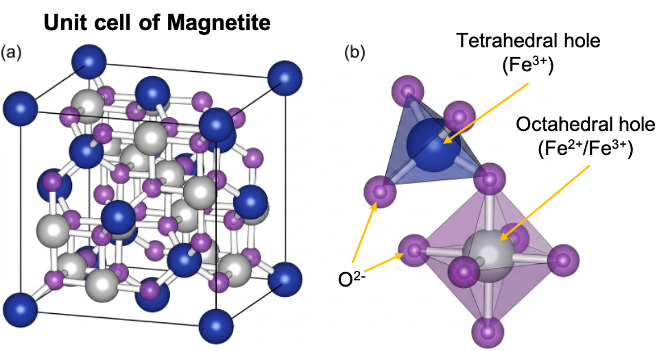
- Ferrimagnetism: In materials such as Fe₃O₄ (magnetite), the spins of neighbouring Fe ions are aligned antiparallel, as in antiferromagnets, but the opposing magnetic moments are unequal. This is because Fe₃O₄ can be represented as Fe3+[Fe2+Fe3+]O4, with Fe3+ occupying tetrahedral holes and both Fe3+ and Fe2+ occupying octahedral holes (see diagram above). Because Fe3+ and Fe2+ ions are present in a 2:1 ratio, the magnetic moments of the Fe3+ ions largely cancel one another, leaving an uncompensated magnetic moment arising from the Fe2+ ions. As a result, the material possesses a non-zero net magnetisation and exhibits domain behaviour and hysteresis similar to those of ferromagnets. In fact, the strongest permanent magnets, such as neodymium magnets, exhibit ferrimagnetism.
-
- Paramagnetism: In materials such as Al and Pt (including O₂ gas), atomic magnetic moments are largely independent in the absence of strong exchange interactions. They align weakly and only temporarily with an applied magnetic field due to thermal agitation, and the magnetisation disappears when the field is removed.
-
- Diamagnetism: In materials such as Cu, Ag and Au (including H2O), there are no permanent magnetic moments from unpaired electrons. An applied magnetic field induces small circulating currents that oppose the applied field, producing a weak, negative magnetisation that is present only while the field is applied. In fact, all materials exhibit diamagnetism to some extent due to Lenz’ law. In paramagnetic and ferromagnetic materials, however, this effect is usually overwhelmed by stronger magnetic mechanisms. Because diamagnetic materials are repelled by magnetic fields, they can be levitated in sufficiently strong magnetic field gradients. A notable example is the levitation of superconductors, which behave as perfect diamagnets due to the Meissner effect.
Question
Explain the hysteresis loop in detail.
Answer
Consider a piece of iron with randomly oriented magnetic domains such that . As
increases from zero, the domains begin to align with the applied field. This initial magnetisation is represented by the dotted curve, which rises rapidly and reaches saturation magnetisation
when all domains are aligned. A common misconception is that
returns to zero when
is subsequently reduced. Instead, the material retains a magnetisation known as the remanent magnetisation
, because the aligned domains remain energetically stable, and only some domains reverse as
decreases to zero. If a negative magnetic field is then applied, more domains begin to reverse and
decreases to zero at
(the coercive field). Beyond this point, a sufficiently strong negative field aligns all domains in the opposite direction, producing the negative saturation magnetisation
. When the negative field is subsequently reduced back to zero, a remanent magnetisation of
remains. Next, increasing
in the positive direction causes the domains to reverse once again. The magnetisation returns to zero at
, and further increases in
eventually bring the material back to the positive saturation magnetisation
, thereby completing the hysteresis loop.
The area enclosed by the hysteresis loop represents the energy dissipated as heat during one complete magnetisation cycle. Consequently, transformer cores are typically made from materials with narrow hysteresis loops to minimise energy losses, whereas permanent magnets are designed to have wide hysteresis loops and large coercivities so that they retain their magnetisation more effectively.
Ultimately, a solid’s magnetic identity is not a static property, but a dynamic equilibrium dictated by this delicate balance between quantum-scale spin ordering and large-scale thermodynamic and electrostatic forces.
Question
What properties of Fe, Co and Ni, compared to Al and Pt, make them ferromagnetic?
Answer
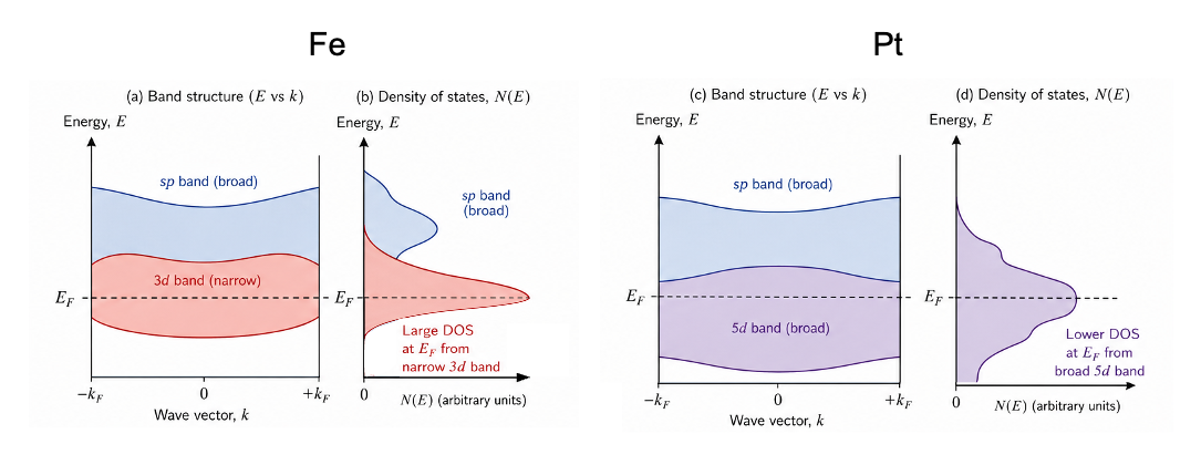
Fe, Co and Ni have partially filled spatially compact 3d orbitals that form smaller overlaps with each other, leading to narrower bands. These narrower bands consist of a large number of available electronic states concentrated near the Fermi level, giving a high density of states (see diagram below). In contrast, the 5d orbitals in Pt are more spatially extended and overlap more strongly, producing broader bands with a lower density of states at the Fermi level. Similarly, the valence s–p bands in Al are relatively broad and have a low density of states at the Fermi level. Consequently, the energy gained from exchange interactions in Fe, Co and Ni through parallel spin alignment exceeds the energy cost associated with the redistribution of electrons between states (the kinetic energy cost of spin polarisation), leading to spontaneous ferromagnetic ordering. An applied magnetic field can then readily enlarge favourably-oriented domains and rotate domain magnetisations, producing a strong net magnetisation.