Navier-Stokes equation

The Navier-Stokes equation is used to describe the motion of a viscous fluid and was named after Claude-Louis Navier, a French scientist, and George Stokes, an Irish scientist. To derive the equation, let’s consider the flow of an incompressible fluid through an infinitesimal cubic control volume* depicted in the diagram below.

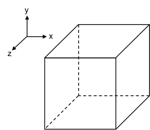
* the control volume here refers to the volume of an object in the fluid.

The x-component of the velocity of the fluid is a function of x, y, z and t, i.e. u_x (x, y, z, t) where t is time. The total differential of u_xis:

$du_x=\frac{\partial u_x}{\partial x}dx+\frac{\partial u_x}{\partial y}dy+\frac{\partial u_x}{\partial z}dz+\frac{\partial u_x}{\partial t}dt$

Dividing the equation by dt and letting dx/dt = u_x, dy/dt = u_y, dz/dt = u_z, we have:

$\frac{du_x}{dt}=u_x\frac{\partial u_x}{\partial x}+u_y\frac{\partial u_x}{\partial y}+u_z\frac{\partial u_x}{\partial z}+\frac{\partial u_x}{\partial t}\; \; \; \; \; \; \; (24)$

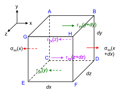
Let’s analyse the hydrostatic and hydrodynamic forces acting on each face of the infinitesimal control volume in the x-direction (see diagram above where point C is the origin). They are summarised as follows:

Face	Force per unit area	Force
BDFH	σ_xx(x + dx)	σ_xx(x + dx)dydz
ACEG	σ_xx(x)	σ_xx(x)dydz
ABHG	τ_yx(y + dy)	τ_yx(y + dy)dxdz
CDFE	τ_yx(y)	τ_yx(y)dxdz
ABDC	τ_zx(z)	τ_zx(z)dxdy
GHFE	τ_zx(z + dz)	τ_zx(z + dz)dxdy

σ_xx = F/A , i.e. the force F acting on a unit area of the x-plane in the x-direction, thereby the double-x subscript. The notation σ_xx(x) refers to σ_xx evaluated at a distance of (x) while σ_xx(x + dx) is evaluated at a distance of (x + dx). A different notation τ is given to the forces that act parallel to the faces of the control volume, e.g. τ_yx(y + dy) is the force acting on a unit area of the y-plane in the x-direction that is evaluated at a distance of (y + dy).

With reference to the defined directions of the forces, F_Hthe sum of hydrostatic and hydrodynamic forces acting on the infinitesimal control volume in the positive x-direction is:

$F_H=\sigma_{xx}(x+dx)dydz-\sigma_{xx}(x)dydz+\tau_{yx}(y+dy)dxdz-\tau_{yx}(y)dxdz +\tau_{zx}(z+dz)dxdy-\tau_{zx}(z)dxdy$

In addition to hydrostatic and hydrodynamic forces, an inertia force F_g (gravitational force) also acts on the infinitesimal control volume in the x-direction:

$F_g=\rho g_xdxdydz$

where ρ is the density of the fluid and g_x is the x-component of the acceleration due to gravity.

The total force F_Tacting on the infinitesimal control volume in the x-direction is therefore:

$F_T=F_H+F_g\; \; \; \; \; \; \; (25)$

Next, by i) substituting F_H and F_g and eq24 in eq25; ii) dividing the substituted equation by dxdydz and iii) letting dx, dy, dz → 0 for an infinitesimal control volume, we have:

$\rho\left ( u_x\frac{\partial u_x}{\partial x} +u_y\frac{\partial u_x}{\partial y}+u_z\frac{\partial u_x}{\partial z} +\frac{\partial u_x}{\partial t} \right )=\frac{\partial \sigma_{xx}}{\partial x} +\frac{\partial \tau_{yx}}{\partial y} +\frac{\partial \tau_{zx}}{\partial z} +\rho g_x\; \; \; \; \; \; \; (26)$

Using the same logic and repeating the above steps, we have for the y-direction and the z-direction:

$\rho\left ( u_x\frac{\partial u_x}{\partial x}+ u_y\frac{\partial u_x}{\partial y}+ u_z\frac{\partial u_x}{\partial z}+\frac{\partial u_y}{\partial t}\right )= \frac{\partial \sigma_{yy}}{\partial y}+\frac{\partial \tau_{zy}}{\partial z}+\frac{\partial \tau_{xy}}{\partial x}+\rho g_y\; \; \; \; \; \; \; (27)$

$\rho\left ( u_x\frac{\partial u_x}{\partial x}+ u_y\frac{\partial u_x}{\partial y}+ u_z\frac{\partial u_x}{\partial z}+\frac{\partial u_z}{\partial t}\right )= \frac{\partial \sigma_{zz}}{\partial z}+\frac{\partial \tau_{xz}}{\partial x}+\frac{\partial \tau_{yz}}{\partial y}+\rho g_z\; \; \; \; \; \; \; (28)$

From the articles on constitutive relation, $\sigma_{ij}=-p\delta_{ij}+\mu\left ( \frac{\partial u_i}{\partial x_j}+\frac{\partial u_j}{\partial x_i}\right )$ . We therefore substitute $\sigma_{xx}=-p+2\mu \frac{\partial u_x}{\partial x}$ , $\tau_{yx}=\mu\left ( \frac{\partial u_x}{\partial y}+\frac{\partial u_y}{\partial x}\right )$ and $\tau_{zx}=\mu\left ( \frac{\partial u_z}{\partial x}+\frac{\partial u_x}{\partial z}\right )$ in eq26, noting that $\frac{\partial u_x}{\partial x}+\frac{\partial u_y}{\partial y}+\frac{\partial u_z}{\partial z}=\nabla\cdot\textbf{\textit{u}}=0$ (see eq14) to give:

$\rho\left ( \frac{\partial u_x}{\partial t}+u_x\frac{\partial u_x}{\partial x} +u_y\frac{\partial u_x}{\partial y}+u_z\frac{\partial u_x}{\partial z} \right )=\rho g_x-\frac{\partial p}{\partial x}+\mu\left ( \frac{\partial^2 u_x}{\partial x^2} +\frac{\partial^2 u_x}{\partial y^2}+\frac{\partial^2 u_x}{\partial z^2}\right )\; \; \; \; \; \; \; (29)$

Using the same logic and repeating the above step for eq27 and eq28, we have:

$\rho\left ( \frac{\partial u_y}{\partial t} +u_x\frac{\partial u_y}{\partial x} +u_y\frac{\partial u_y}{\partial y}+u_z\frac{\partial u_y}{\partial z} \right )=\rho g_y-\frac{\partial p}{\partial y}+\mu\left ( \frac{\partial ^2u_y}{\partial x^2}+\frac{\partial ^2u_y}{\partial y^2} +\frac{\partial ^2u_y}{\partial z^2}\right )\; \; \; \; \; \; \; (30)$

$\rho\left ( \frac{\partial u_z}{\partial t} +u_x\frac{\partial u_z}{\partial x} +u_y\frac{\partial u_z}{\partial y}+u_z\frac{\partial u_z}{\partial z} \right )=\rho g_z-\frac{\partial p}{\partial z}+\mu\left ( \frac{\partial ^2u_z}{\partial x^2}+\frac{\partial ^2u_z}{\partial y^2} +\frac{\partial ^2u_z}{\partial z^2}\right )\; \; \; \; \; \; \; (31)$

Eq29, eq30 and eq31 are the Cartesian form of the Navier-Stokes equations, which when multiplied throughout by the unit vectors $\hat{x}$ , $\hat{y}$ and $\hat{z}$ respectively and summed, becomes the vector form:

$\rho\frac{D\textbf{\textit{u}}}{Dt}=-\nabla p+\rho g+\mu \nabla^2\textbf{\textit{u}}\; \; \; \; \; \; \; (32)$

where

$\nabla^2\textbf{\textit{u}}=\nabla^2 u_x\hat{x}+\nabla^2 u_y\hat{y}+\nabla^2 u_z\hat{z}$

$\frac{D}{Dt}$ is the convective derivative defined as $\frac{D}{Dt}=\frac{\partial }{\partial t}+\textbf{\textit{u}}\cdot \nabla$

$\nabla$ is the gradient defined as $\nabla =\hat{x}\frac{\partial }{\partial x}+\hat{y}\frac{\partial }{\partial y}+\hat{z}\frac{\partial }{\partial z}$