Heisenberg’s uncertainty principle

Heisenberg’s uncertainty principle states that the position and momentum of a particle cannot be determined simultaneously with unlimited precision. It was developed by Werner Heisenberg, a German physicist, in 1927 and is expressed mathematically as:

$\Delta p_x\Delta x\geq \frac{\hbar}{2}$

where $\Delta p_x$ is the uncertainty in the x-component of a particle’s momentum, $\Delta x$ is the uncertainty in the particle’s position along the x-axis, and $\hbar=\frac{h}{2\pi}$ .

In other words, the product of the uncertainty in measuring a particle’s momentum and the uncertainty in the simultaneous measuring of the particle’s position is never less than $\hbar/2$ (see here for proof). It is important to note that the uncertainties in the measurements are not due to the limitation of measuring devices but an inherent property of nature.

To explain the uncertainty principle, we turn to de Broglie’s hypothesis, which states that all matter behaves like waves. For an electron, its wave property is described by a wave function, e.g. $\psi=Ae^{ikx}$ , which has a well-defined wavelength $\lambda=\frac{2\pi}{k}$ (since $Ae^{ik\left ( x+\frac{2\pi}{k} \right )}=Ae^{ikx}$ ) and hence a precisely determined momentum $p=\frac{h}{\lambda}=k\hbar$ . Furthermore, the position of the electron, according to the Born interpretation, is given by the probability density $\left | \psi \right |^2$ where

$\left | \psi \right |^2=\psi^*\psi=Ae^{-ikx}Ae^{ikx}=A^2$

The equation above shows that the probability density of the electron is uniform, i.e. the electron has equal probability to be found anywhere along the x-axis. If an electron’s momentum is precisely specified, its location cannot simultaneously be determined.

For the reverse argument, where the position is precisely defined, let’s start with an electron with a wave function, where the wavelength is precisely defined, e.g. $cos\pi x$ (represented by the red curve in diagram I below).

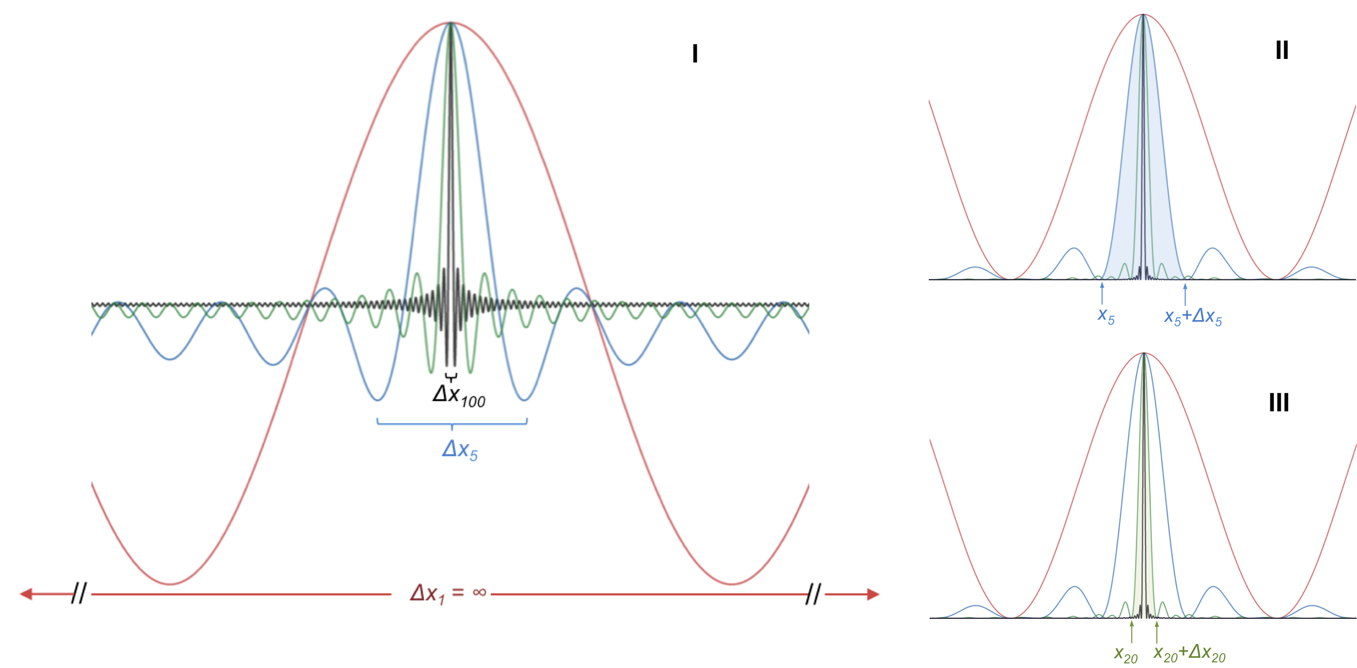
If we linearly add another wave function with a different wavelength $cos2\pi x$ to $cos\pi x$ and divide the sum by two* to maintain the same amplitude as $cos\pi x$ , we have a new wave function $y=\frac{1}{2}cos\pi x+\frac{1}{2}cos2\pi x$ or $\sum_{n=1}^{N}\frac{cosn\pi x}{N}$ where N = 2. This is equivalent to the interference pattern of two superimposed wave functions. If we continue to superimpose the first wave function with more wave functions, each of different wavelength, we end up with the blue curve, the green curve and the black curve, for N =5, N = 20 and N = 100 respectively. It is evident from diagram I that as more wave functions of different wavelengths are linearly added to the first wave function, the spread of the resultant wave function becomes narrower.

* this is done for convenience, so that the resultant curve can fit within our view.

For the N = 5 wave function, the probability of locating the electron within a certain percentage P is $\int \left | \psi \right |^2dx$ , which is the area under the blue curve from x₅ to x+Δx₅ (diagram II). Notice that all curves in diagram II are above the x-axis since they represent the square of the respective wave functions. For the N = 20 wave function, let’s assume that the probability of locating the electron within the same percentage is approximately the area under the green curve from x₂₀ to Δx₂₀ in diagram III (note that the amplitude of the N = 20 function in the diagram is normalised for convenience; rightfully, it is very much higher than the amplitude of the N =5 function, and hence the areas under both peaks are comparable). Clearly, the interval x₂₀ to x+Δx₂₀ is shorter than the interval x₅ to x+Δx₅. Hence, we can locate the electron, with a certain probability P, within a smaller interval as N increases, i.e. the uncertainty in locating the electron becomes smaller as N increases. However, the resultant wave functions of N =5 and N = 20 now consist of 5 and 20 distinct wavelengths respectively. Since each wavelength represent a specific value of momentum, a wave function with a wider spread of wavelengths leads to a greater uncertainty of momentum. In the limit of N → ∞ , we have a precisely localised electron but a completely unpredictable momentum.

Question

The speed of an electron in a one-dimensional space is measured, within 3% accuracy, as 2.20 x 10⁶ m/s. What is the length of the space?

Answer

The minimum uncertainty in the position of the electron is:

$\Delta x\geq \frac{\hbar}{2m\Delta v_x}=\frac{1.055\times10^{-34}}{2\times9.11\times10^{-31}\times0.03\times2.20\times10^6}=8.8\times10^{-10}\, m$

If we assume that there is absolute certainty that the electron is not outside the region of space, the uncertainty in position of the electron must be attributed to the length of space.

Heisenberg’s uncertainty principle

Question

Answer

Next article: Nuclear spin

Previous article: Hund’s rule

Content page of intermediate quantum chemistry

Content page of intermediate chemistry

Main content page

Leave a Reply Cancel reply