Liquid-liquid phase diagrams are graphical representations that show the conditions under which two (or more) partially or fully immiscible liquids coexist in equilibrium. The most common type of liquid-liquid phase diagram is the temperature-composition diagram.
A typical temperature-composition diagram of two partially miscible liquids features a binodal curve (with two nodes at the ends of a tie-line) that divides the diagram into two regions (see diagram below). The region outside the curve corresponds to a single liquid phase, while the area enclosed by the curve represents a two-phase region, where the liquids separate into two immiscible layers
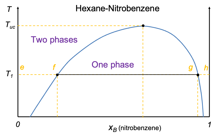
To interpret this diagram, consider starting at point e, which represents pure liquid A (hexane) at a fixed temperature and 1 atm. As small amounts of liquid B (nitrobenzene) are gradually added, it dissolves completely in A to form a single-phase solution between e and f. Upon further addition of B, the system reaches the limit of mutual solubility, and phase separation occurs (between points f and g, the system exists as two liquid phases). Along the tie line connecting f and g, each end corresponds to the composition of one of the two coexisting phases. A mixture composition closer to f indicates that the phase richer in A is more abundant, while the phase richer in B (composition at g) is less abundant. The opposite holds for mixtures closer to g. The lever rule can be applied to determine the relative amounts of each phase. At point g, enough B has been added to dissolve all of A, resulting in a saturated single-phase solution of A in B. Further addition of B beyond this point leads to continuous dilution of A, and the system remains in the single-phase region until pure B is reached at point h, where
.
A liquid-liquid phase diagram like the one above is constructed with empirical data. It is interesting to note that the compositions of the two phases at equilibrium for the hexane-nitrobenzene system vary with temperature. The narrowing of the curve at higher temperatures indicates an increasing miscibility of the two components as temperature rises. The upper critical solution temperature is the temperature above which the system exists as a single phase, with the two liquids miscible in all proportions.
Some binary liquid systems exhibit greater miscibility as temperature decreases (see diagram below). An example is the water–triethylamine system, in which the two components form a weak complex at lower temperatures. In such cases, a lower critical solution temperature marks the temperature below which the system becomes fully miscible and exists as a single phase.
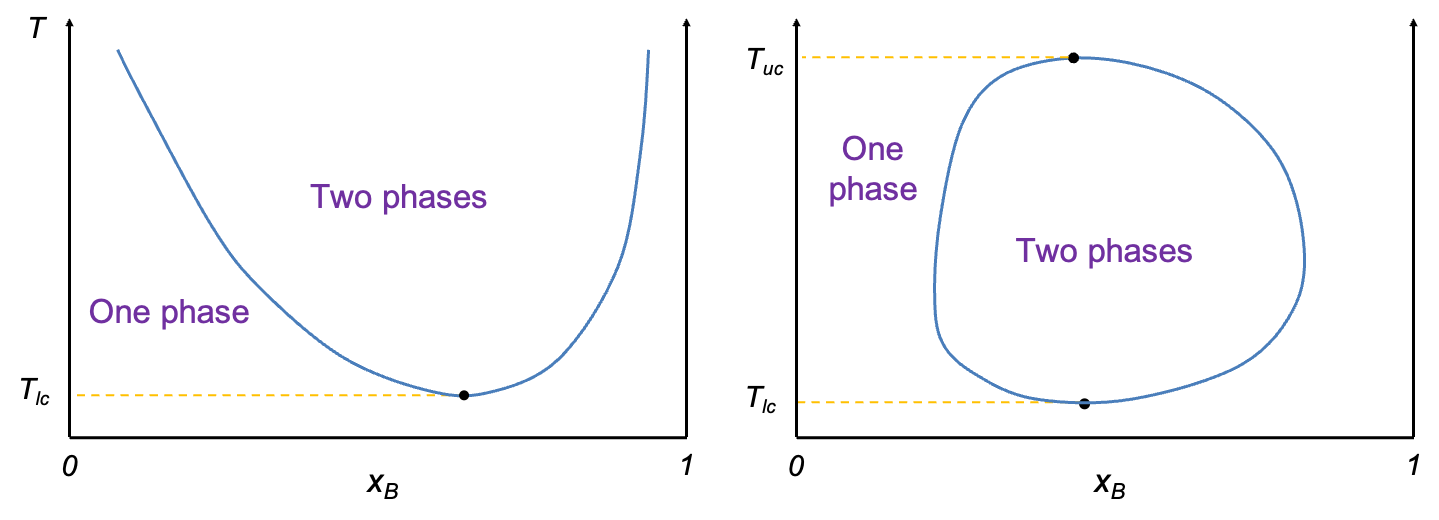
Occasionally, a system displays a combination of both behaviours, exhibiting both an upper and a lower critical solution temperature (see diagram above). In such systems, the components are completely miscible at both high and low temperatures, but become partially miscible over an intermediate temperature range. This results in a closed-loop miscibility gap on the temperature–composition diagram, bounded above by the upper critical solution temperature and below by the lower critical solution temperature. The unusual phase behaviour is typically due to competing molecular interactions, such as complex formation at low temperatures and thermal disruption at higher temperatures. Examples include nicotine–water and m-toluidine–glycerol systems.
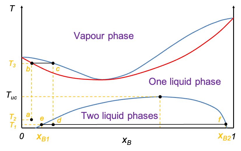
Liquid–liquid diagrams are commonly used in extractive distillation processes, where the goal is to exploit both vapour–liquid equilibrium and liquid–liquid immiscibility to achieve better separation. The diagram above shows a mixture of two partially miscible liquids that form a low-boiling azeotrope. An example is the water–isobutanol system. If a water–isobutanol mixture of composition at point a is heated from to
, the resulting vapour, upon cooling to
will condense into a distillate consisting of two phases: one with composition
and the other
.
Beyond separation, liquid–liquid diagrams also play a crucial role in other scientific fields. In polymer blends and materials engineering, they help predict phase compatibility and guide the design of homogeneous or phase-separated materials with tailored properties. In food science, liquid–liquid behaviour underpins the formation and stabilisation of oil–water emulsions, which are essential in products like dressings, creams and sauces. Similarly, in environmental science, such diagrams aid in understanding the partitioning of pollutants between aqueous and organic phases, which is key to modelling contaminant transport and designing remediation strategies.