Bell’s inequality

Bell’s inequality, developed by John Bell in 1964, is a non-equal relation (between two expressions) that is based on the ERP paradox. It provides a way to determine whether quantum theory or the EPR paradox is correct. Bell suggested a unique way of measuring the spins of two spin- $\frac{1}{2}$ particles, which are generated from the decay of a spin-0 particle at rest: the two particles are to be passed through two Stern-Gerlach devices, each oriented along one of three non-orthogonal coplanar axes, which are specified by the unit vectors $\boldsymbol{a}$ , $\boldsymbol{b}$ and $\boldsymbol{c}$ .

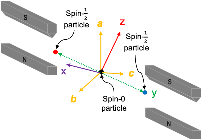
The average values of the product of the spins in units of $\frac{\hbar}{2}$ (denoted by $P(\boldsymbol{a},\boldsymbol{b})$ , $P(\boldsymbol{b},\boldsymbol{c})$ , and $P(\boldsymbol{a},\boldsymbol{c})$ ) are then calculated. As derived in an earlier article (see eq227), quantum mechanics expresses the average values as:

$P(\boldsymbol{a},\boldsymbol{b})=P(\boldsymbol{b},\boldsymbol{c})=P(\boldsymbol{a},\boldsymbol{c})=-cos\theta\; \; \; \; \; \; \; \; 228$

For the ERP paradox, let’s equate a spin-up measurement to +1 and a spin-down measurement to -1. The average value of the product of the measured spins, for example in the $\boldsymbol{a}$ and $\boldsymbol{b}$ directions, is:

$P(\boldsymbol{a},\boldsymbol{b})=\int_{\lambda_i}^{\lambda_f}\rho(\lambda)A(\boldsymbol{a},\lambda)B(\boldsymbol{b},\lambda)d\lambda\; \; \; \; \; \; \; \; 229$

where

i) $\lambda$ is a hidden variable.

ii) $\rho(\lambda)$ is the probability density that is a function of $\lambda$ , with $\int_{\lambda_i}^{\lambda_f}\rho(\lambda)d\lambda=1$ and $\rho(\lambda)\geq 0$ .

iii) $A(\boldsymbol{a},\lambda)$ is a function of the axis of measurement and $\lambda$ . It is associated with the measurement made by the first Stern-Gerlach device, and has output values of $\pm1$ .

iv) $B(\boldsymbol{b},\lambda)$ is a function of the axis of measurement and $\lambda$ . It is associated with the measurement made by the second Stern-Gerlach device, and has output values of $\pm1$ .

From experiments, we know that

$A(\boldsymbol{a},\lambda)=-B(\boldsymbol{b},\lambda)\; \; \; \; \; \; \; \; 230$

Substitute eq230 in eq229

$P(\boldsymbol{a},\boldsymbol{b})=-\int_{\lambda_i}^{\lambda_f}\rho(\lambda)A(\boldsymbol{a},\lambda)A(\boldsymbol{b},\lambda)d\lambda\; \; \; \; \; \; \; \; 231$

Similarly, $P(\boldsymbol{a},\boldsymbol{c})=-\int_{\lambda_i}^{\lambda_f}\rho(\lambda)A(\boldsymbol{a},\lambda)A(\boldsymbol{c},\lambda)d\lambda$ and $P(\boldsymbol{b},\boldsymbol{c})=-\int_{\lambda_i}^{\lambda_f}\rho(\lambda)A(\boldsymbol{b},\lambda)B(\boldsymbol{c},\lambda)d\lambda$ . Therefore,

$P(\boldsymbol{a},\boldsymbol{b})-P(\boldsymbol{a},\boldsymbol{c})=-\int_{\lambda_i}^{\lambda_f}\rho(\lambda)A(\boldsymbol{a},\lambda)A(\boldsymbol{b},\lambda)d\lambda+\int_{\lambda_i}^{\lambda_f}\rho(\lambda)A(\boldsymbol{a},\lambda)A(\boldsymbol{c},\lambda)d\lambda$

Since $[A(\boldsymbol{b},\lambda)]^{2}=1$ , we can rearrange the above equation to

$P(\boldsymbol{a},\boldsymbol{b})-P(\boldsymbol{a},\boldsymbol{c})=-\int_{\lambda_i}^{\lambda_f}\rho(\lambda)[1-A(\boldsymbol{b},\lambda)A(\boldsymbol{c},\lambda)]A(\boldsymbol{a},\lambda)A(\boldsymbol{b},\lambda)d\lambda$

Taking the absolute value on both sides of the above equation and using the relation $\left | \int f(t)dt\right |\leq \int \left | f(t) \right |dt$

$\vert P(\boldsymbol{a},\boldsymbol{b})-P(\boldsymbol{a},\boldsymbol{c})\vert\leq \int_{\lambda_i}^{\lambda_f}\left | \rho(\lambda)[1-A(\boldsymbol{b},\lambda)A(\boldsymbol{c},\lambda)]\right | \vert A(\boldsymbol{a},\lambda)A(\boldsymbol{b},\lambda)\vert d\lambda$

Question

Why is $\left | \int_{a}^{b}f(t)dt \right |\leq \int_{a}^{b}\vert f(t)\vert dt$ ?

Answer

For all $t\in [a,\cdots,b]$ , we have $-\vert f(t)\vert\leq f(t)\leq \vert f(t)\vert$ . Therefore, $-\int_{a}^{b}\vert f(t)\vert dt\leq\int_{a}^{b} f(t) dt\leq \int_{a}^{b}\vert f(t)\vert dt$ or simply $\left | \int_{a}^{b}f(t)dt \right |\leq \int_{a}^{b}\vert f(t)\vert dt$ , where we have use the identity of $\vert x\vert\leq a\; \; \; \; \Leftrightarrow \; \; \; \; -a\leq x\leq a$ .

Since $\vert A(\boldsymbol{a},\lambda)A(\boldsymbol{b},\lambda)\vert =1$

Since $\rho(\lambda)\geq 0$ and $1-A(\boldsymbol{b},\lambda)A(\boldsymbol{c},\lambda)\geq 0$ , we can ignore the absolute value sign on RHS of the above equation:

$\vert P(\boldsymbol{a},\boldsymbol{b})-P(\boldsymbol{a},\boldsymbol{c})\vert\leq \int_{\lambda_i}^{\lambda_f} \rho(\lambda)d\lambda-\int_{\lambda_i}^{\lambda_f}\rho(\lambda)A(\boldsymbol{b},\lambda)A(\boldsymbol{c},\lambda) d\lambda$

Substituting $\int_{\lambda_i}^{\lambda_f} \rho(\lambda)d\lambda=1$ and $P(\boldsymbol{b},\boldsymbol{c})=-\int_{\lambda_i}^{\lambda_f}\rho(\lambda)A(\boldsymbol{b},\lambda)A(\boldsymbol{c},\lambda) d\lambda$ into the above equation gives

$\vert P(\boldsymbol{a},\boldsymbol{b})-P(\boldsymbol{a},\boldsymbol{c})\vert\leq 1+P(\boldsymbol{b},\boldsymbol{c})\; \; \; \; \; \; \; \; 232$

Eq232 is the Bell’s inequality, which is based on the ERP paradox.

To show that quantum mechanics is incompatible with Bell’s inequality, we let $\angle \boldsymbol{a}\boldsymbol{c}=\angle \boldsymbol{b}\boldsymbol{c}=45^{\circ}$ , i.e. $\boldsymbol{c}$ bisects $\angle \boldsymbol{a}\boldsymbol{b}$ . From eq228,

$P(\boldsymbol{a},\boldsymbol{b})=-cos90^{\circ}=0\; \; \; \; \; \; \; \; 233$

$P(\boldsymbol{b},\boldsymbol{c})=P(\boldsymbol{a},\boldsymbol{c})=-cos45^{\circ}=-\frac{1}{\sqrt{2}}\; \; \; \; \; \; \; \; 234$

Substituting eq233 and eq234 in eq232 yields $\frac{1}{\sqrt{2}}\leq1-\frac{1}{\sqrt{2}}$ , which is inconsistent with Bell’s inequality. Therefore, it is possible to experimentally measure the spins of the two particles at non-orthogonal angles to test the predictions of quantum theory versus the ERP paradox. In fact, the results of all experiments conducted at non-orthogonal angles were in agreement with quantum mechanics. This implies that all local hidden-variable hypotheses are invalid.

Bell’s inequality

Question

Answer

Next article: quantum key distribution

Previous article: einstein-podolsky-rosen paradox

Content page of quantum mechanics

Content page of advanced chemistry

Main content page

Leave a Reply Cancel reply