Pauli matrices

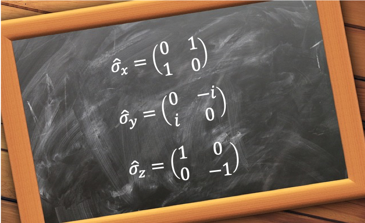
Pauli matrices are matrix representations of the spin operators $\small \hat{S}_x$ , $\small \hat{S}_y$ and $\small \hat{S}_z$ .

To derive the Pauli matrices, we let $\small \alpha$ and $\small \beta$ be basis vectors representing the electron spin eigenstates of $\small \vert s=1/2,m_s=1/2\rangle$ and $\small \vert s=1/2,m_s=-1/2\rangle$ respectively, with the following assignments:

$\small \alpha=\begin{pmatrix} 1\\0 \end{pmatrix}\; \; \; \; \; \; \beta=\begin{pmatrix} 0\\1 \end{pmatrix}$

The general state of an electron can then be written as a linear combination of the two spin states:

$\small \chi=c_1\alpha+c_2\beta\; \; \; \; \; \; \; \; 171$

where $\small \vert c_1\vert^{2}$ is the probability of finding the electron with the state $\small \vert s=1/2,m_s=1/2\rangle$ , and $\small \vert c_2\vert^{2}$ is the probability of finding the electron with the state $\small \vert s=1/2,m_s=-1/2\rangle$ , with

$\small \vert c_1\vert^{2}+\vert c_2\vert^{2}=1\; \; \; \; \; \; \; \; 172$

Having defined the two eigenstates, we can work out the corresponding matrix representation of $\small \hat{S}^{2}$ using eq169 by letting $\small \hat{S}^{2}=\begin{pmatrix} a &b \\ c &d \end{pmatrix}$ :

$\small \begin{pmatrix} a &b \\ c &d \end{pmatrix}\begin{pmatrix} 1\\0 \end{pmatrix}=\frac{3}{4}\hbar^{2}\begin{pmatrix} 1\\0 \end{pmatrix}\; \; \; \; \; \Rightarrow \; \; \; \; \; \begin{pmatrix} a\\c \end{pmatrix}=\begin{pmatrix} \frac{3}{4}\hbar^{2}\\ 0 \end{pmatrix}$

$\small \begin{pmatrix} a &b \\ c &d \end{pmatrix}\begin{pmatrix} 0\\1 \end{pmatrix}=\frac{3}{4}\hbar^{2}\begin{pmatrix} 0\\1 \end{pmatrix}\; \; \; \; \; \Rightarrow \; \; \; \; \; \begin{pmatrix} b\\d \end{pmatrix}=\begin{pmatrix} 0\\ \frac{3}{4}\hbar^{2} \end{pmatrix}$

So,

$\small \hat{S}^{2}=\frac{3}{4}\hbar^{2}\begin{pmatrix} 1 &0 \\ 0 &1 \end{pmatrix}\; \; \; \; \; \; \; \; 173$

Similarly, using eq168 for $\small \hat{S}_z$ , we have

$\small \hat{S}_z=\frac{\hbar}{2}\begin{pmatrix} 1 &0 \\ 0 &-1 \end{pmatrix}\; \; \; \; \; \; \; \; 174$

For $\small \hat{S}_x$ and $\small \hat{S}_y$ , we make use of eq170 where

$\small \hat{S}_+\begin{pmatrix} 0\\1 \end{pmatrix}=\hbar\sqrt{\frac{3}{4}+\frac{1}{2}\left ( -\frac{1}{2}+1 \right )}\begin{pmatrix} 1\\0 \end{pmatrix}=\hbar\begin{pmatrix} 1\\0 \end{pmatrix}\; \; \; \; \; \; \Rightarrow \; \; \; \; \; \hat{S}_+=\hbar\begin{pmatrix} 0 &1 \\ 0& 0 \end{pmatrix}\; \; \; \; \; \; \; \; 175$

$\small \hat{S}_-\begin{pmatrix} 1\\0 \end{pmatrix}=\hbar\sqrt{\frac{3}{4}-\frac{1}{2}\left (\frac{1}{2}-1 \right )}\begin{pmatrix} 0\\1 \end{pmatrix}=\hbar\begin{pmatrix} 0\\1 \end{pmatrix}\; \; \; \; \; \; \Rightarrow \; \; \; \; \; \hat{S}_-=\hbar\begin{pmatrix} 0 &0 \\ 1& 0 \end{pmatrix}\; \; \; \; \; \; \; \; 176$

Since $\small \hat{S}_\pm=\hat{S}_x\pm i\hat{S}_y$ , we have $\small \hat{S}_x=\hat{S}_+-i\hat{S}_y=\hat{S}_+-(\hat{S}_x-\hat{S}_-)$ or $\small \hat{S}_x=\frac{\hat{S}_++\hat{S}_-}{2}$ . Similarly, $\small \hat{S}_y=\frac{\hat{S}_+-\hat{S}_-}{2i}$ . Using eq175 and eq176,

$\small \hat{S}_x=\frac{\hbar}{2}\begin{pmatrix} 0 &1 \\ 1 & 0 \end{pmatrix}\; \; \; \; \; \; \; \; 177$

$\small \hat{S}_y=\frac{\hbar}{2}\begin{pmatrix} 0 &-i \\ i & 0 \end{pmatrix}\; \; \; \; \; \; \; \; 178$

In an earlier article, when we constructed quantum orbital angular momentum component operators $\small \hat{L}_x$ , $\small \hat{L}_y$ and $\small \hat{L}_z$ , we replaced the position and linear momentum components of the classical angular momentum components $\small L_x$ , $\small L_y$ and $\small L_z$ with their corresponding operators. We also suggested that we could have constructed an angular momentum operator using $\small \boldsymbol{\mathit{L}}=\boldsymbol{\mathit{i}}L_x+\boldsymbol{\mathit{j}}L_y+\boldsymbol{\mathit{k}}L_z$ , such that $\small \hat{\boldsymbol{\mathit{L}}}=\boldsymbol{\mathit{i}}\hat{L}_x+\boldsymbol{\mathit{j}}\hat{L}_y+\boldsymbol{\mathit{k}}\hat{L}_z$ , but for certain reasons chose to construct $\small \hat{L}^{2}$ instead. For electron spin, it is useful to construct the spin operator using that suggestion:

$\small \hat{\boldsymbol{\mathit{S}}}=\boldsymbol{\mathit{i}}\hat{S}_x+\boldsymbol{\mathit{j}}\hat{S}_y+\boldsymbol{\mathit{k}}\hat{S}_z=\frac{\hbar}{2}\hat{\boldsymbol{\mathit{\sigma}}}\; \; \; \; \; \; \; \; 179$

where $\small \hat{\boldsymbol{\mathit{\sigma}}}=\boldsymbol{\mathit{i}}\hat{\sigma}_x+\boldsymbol{\mathit{j}}\hat{\sigma}_y+\boldsymbol{\mathit{k}}\hat{\sigma}_z$ , with

$\small \hat{\sigma}_x=\begin{pmatrix} 0 &1 \\ 1 &0 \end{pmatrix},\; \; \; \; \;\hat{\sigma}_y=\begin{pmatrix} 0 &-i \\ i &0 \end{pmatrix},\; \; \; \; \;\hat{\sigma}_z=\begin{pmatrix} 1 &0 \\ 0 &-1 \end{pmatrix}\; \; \; \; \; \; \; \; 180$

$\small \hat{\sigma}_x$ , $\small \hat{\sigma}_y$ and $\small \hat{\sigma}_z$ are called Pauli matrices. They represent observables and are Hermitian (the complex conjugate of each matrix returns the same matrix). Eq179 and eq180 are used to analyse the results of successive Stern-Gerlach experiments.

Question

Show that $\small [\hat{L}^{2},\hat{\boldsymbol{\mathit{L}}}\cdot\hat{\boldsymbol{\mathit{S}}}]=0$ and $\small [\hat{S}^{2},\hat{\boldsymbol{\mathit{L}}}\cdot\hat{\boldsymbol{\mathit{S}}}]=0$ but $\small \left [ \hat{{L}^{2}}^{T},\hat{\boldsymbol{\mathit{L}}_1}\cdot\hat{\boldsymbol{\mathit{S}}_1}+\hat{\boldsymbol{\mathit{L}}_2}\cdot\hat{\boldsymbol{\mathit{S}}_2}\right ]\neq 0$ .

Answer

For $\small \left [ \hat{L}^{2},\hat{\boldsymbol{\mathit{L}}}\cdot\hat{\boldsymbol{\mathit{S}}}\right ]$ , substitute in $\small \hat{\boldsymbol{\mathit{L}}}=\boldsymbol{\mathit{i}}\hat{L}_x+\boldsymbol{\mathit{j}}\hat{L}_y+\boldsymbol{\mathit{k}}\hat{L}_z$ and $\small \hat{\boldsymbol{\mathit{S}}}=\boldsymbol{\mathit{i}}\hat{S}_x+\boldsymbol{\mathit{j}}\hat{S}_y+\boldsymbol{\mathit{k}}\hat{S}_z$ and expand the expression. From eq102, $\small \hat{L}^{2}$ commutes with all components of $\small \hat{\boldsymbol{\mathit{L}}}$ ; and also all components of $\small \hat{\boldsymbol{\mathit{S}}}$ because orbital angular momentum operators and spin angular momentum operators act on different vector spaces. Thus, $\small \left [ \hat{L}^{2},\hat{\boldsymbol{\mathit{L}}}\cdot\hat{\boldsymbol{\mathit{S}}}\right ]=0$ . Similarly, from eq165, eq166 and eq167, $\small \hat{S}^{2}$ commutes with all components of $\small \hat{\boldsymbol{\mathit{L}}}$ and $\small \hat{\boldsymbol{\mathit{S}}}$ and so $\small \left [ \hat{S}^{2},\hat{\boldsymbol{\mathit{L}}}\cdot\hat{\boldsymbol{\mathit{S}}}\right ]=0$ .

Now,

$\small \hat{{L}^{2}}^{T}=\hat{\boldsymbol{\mathit{L}}}^{T}\cdot\hat{\boldsymbol{\mathit{L}}}^{T}=\left (\hat{\boldsymbol{\mathit{L}}_1}+\hat{\boldsymbol{\mathit{L}}_2}\right )\cdot\left (\hat{\boldsymbol{\mathit{L}}_1}+\hat{\boldsymbol{\mathit{L}}_2}\right )=\hat{L}_{1}^{\: 2} +\hat{L}_{2}^{\: 2}+2\left (\hat{\boldsymbol{\mathit{L}}_1}\cdot\hat{\boldsymbol{\mathit{L}}_2}\right ) \; \; \; \; \; \; \; \; 181$

Substituting eq181 in $\small \left [{\hat{L^{2}}^{T}},\hat{\boldsymbol{\mathit{L}}_1}\cdot\hat{\boldsymbol{\mathit{S}}_1}+\hat{\boldsymbol{\mathit{L}}_2}\cdot\hat{\boldsymbol{\mathit{S}}_2}\right ]\neq 0$ and expanding the expression, we find, after some algebra, that

$\small \left [{\hat{L^{2}}^{T}},\hat{\boldsymbol{\mathit{L}}_1}\cdot\hat{\boldsymbol{\mathit{S}}_1}+\hat{\boldsymbol{\mathit{L}}_2}\cdot\hat{\boldsymbol{\mathit{S}}_2}\right ]\neq 0\; \; \; \; \; \; \; \; 182$

Similarly,

$\left [ \hat{{S}^2}^T,\hat{\boldsymbol{\mathit{L}}}_1\cdot\hat{\boldsymbol{\mathit{S}}}_1+\hat{\boldsymbol{\mathit{L}}}_2\cdot\hat{\boldsymbol{\mathit{S}}}_2\right ]\neq0\; \; \; \; \; \; \; \; 182a$

Question

Next article: Sequential Stern-Gerlach experiments

Previous article: spin angular momentum

Content page of quantum mechanics

Content page of advanced chemistry

Main content page

Leave a Reply Cancel reply