A sequential Stern-Gerlach experiment involves passing a spin- particle through multiple inhomogeneous magnetic fields, each of a certain orientation. In the first example, a beam of spin-
particles, e.g. silver atoms, undergoes a first measurement as it passes through an inhomogeneous magnetic field, which is parallel to the
-axis (see diagram below).
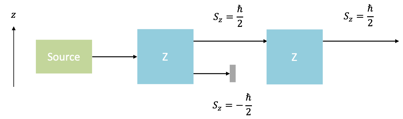
The beam is split into two, and the beam is allowed to travel through another inhomogeneous magnetic field, which is also
-directional (the
beam is blocked). The general state
of the valence silver electron prior to passing through the first magnetic field is given by eq171:
where and
are basis vectors representing the electron spin eigenstates of
and
respectively;
is the probability of finding the electron with the state
, and
is the probability of finding the electron with the state
, with
.
Since the direction of the first magnetic field is arbitrary assigned and the beam of silver atoms emerging from the source is not polarised, we have equal probability of silver atoms with valence electrons in each eigenstate emerging, i.e. . Noting the orthonormality of basis vectors, the expectation value of
with reference to eq168 is:
The state of the valence silver electron entering the second magnetic field is
, where
and
. Therefore, the expectation value of
is
.
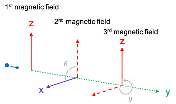
For the second example, the beam emerging from the first magnetic field is passed through a second magnetic field that is rotated 90o, i.e. in the
-direction (see diagram below).

To determine the result of the second measurement, we must express the state of the valence electron in the beam in terms of
and
, or in general where the second magnetic field is rotated parallel to an arbitrary direction
(
is the unit vector in spherical coordinates, i.e.
), in terms of
and
.

Question
How do we derive the unit vector in spherical coordinates?
Answer
Substitute eq77 in the definition of a unit vector,
In other words, we need eq171 to be in the form:
This implies that we have to construct the operator , which acts on the component of spin angular momentum along
. To do so, we take the projection of
onto
:
Hence, the operator is
Substituting eq174, eq177 and eq178 in the above equation to further construct in matrix form,
The eigenvalue equation is:
where is the eigenvalue; and the corresponding characteristic equation is:
Substitute eq183 and eq186 in eq185,
So,
Since and
, we have
Substituting the above equation in and using
Question
Show that .
Answer
If , we have
.
Substitute eq188 in
Therefore, eq183 becomes:
Note that we could have equally used in eq187 to arrive at eq188 and eq189. Using eq188, the probability of measuring the
state is
Using eq189, the probability of measuring the state is
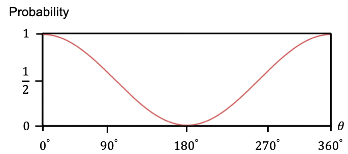
Therefore, we observe that the beam is split equally into two beams by the second magnetic field. Using the same logic, the
beam will again split into two beams by the third magnetic field:
In general, the probability of observing the state is depicted in the graph below.
Question
Do eq188 and eq189 apply to the output of the beam passing through the second magnetic field in the first example?
Answer
Yes. In the first example, and
.