Electronic selection rules for molecules are quantum-mechanical conditions (based on changes in quantum numbers and symmetry) that determine whether transition between energy levels in the molecules are allowed or forbidden.
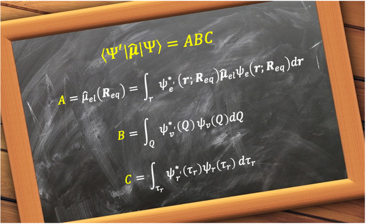
According to the time-dependent perturbation theory, the transition probability between the initial and final states, and
, of a molecule is proportional to the square of the matrix element
, where
is the operator for the molecule’s electric dipole moment.
Consider a homonuclear diatomic molecule. Although it has no permanent dipole moment in a stationary state, it can acquire a transient, time-dependent dipole moment (just as an atom does) when interacting with oscillating incident radiation. Like multi-electron atoms, and
must satisfy the Pauli exclusion principle and can be represented by Slater determinants built from orthogonal spin-orbitals
, with
and
being the spatial and spin wavefunctions respectively, and
. Since the dipole moment operator does not act on the spin wavefunctions, which are identical for the initial and final states, the total spin quantum number does not change, i.e.
.
The selections rules involving angular momentum are determined using the two vanishing integral rules in group theory:
Rule 1
If and
transform according to two different non-equivalent irreducible representations
and
respectively, the integral of their product over all space is necessarily zero
Rule 2
If a function transforms according to an irreducible representation that is not the totally symmetric representation of a group, its integral over all space is necessarily zero
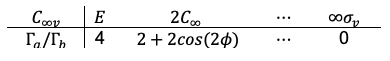
For linear molecules belonging to the point group (see this link for details), the electric dipole moment operator can be resolved into parallel and perpendicular components and transforms according to either the basis function
or the pair
, the latter forming a linear combination of
and
. If the operator transforms as
, then the product
in
transforms according to a direct product representation. In this case, the product transforms as the same irreducible representation as
, since
transforms as the totally symmetric irreducible representation
. Therefore, Rule 1 requires that the initial and final states transform according to the same irreducible representation (
and
) for the integral to be non-zero. This also implies that the transition
is forbidden. Since states transforming as
correspond to
, it follows that
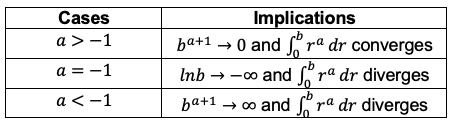
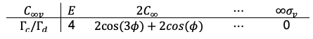
If the dipole moment operator transforms as , we have the following cases:
Case 1: with
The direct product of is
or
, both corresponding to the reducible representation
where we have used the identity .
Decomposing the reducible representation gives: . Since
(see this link for proof), the matrix element
is non-zero according to Rule 2 because it includes the term
.
Case 2: with
The direct product of is
or
, both corresponding to the reducible representation
where we have used the identity .
Decomposing the reducible representation gives: . Since
, the matrix element
is zero according to Rule 2. In fact, if
or
, the character for the rotation operator is always
. Hence,
, for
, will never include the
term, which is necessary for the
component to exist.
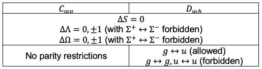
Therefore, the selection rules involving are:
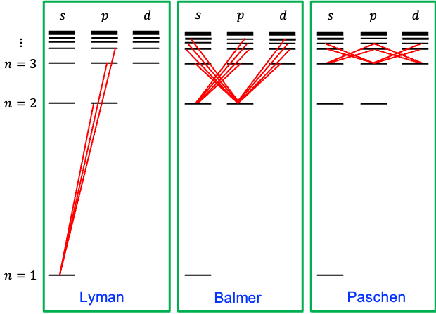
For linear molecules, becomes
(see this link for explanation), where
is the projection of the total electronic angular momentum onto the molecular axis.
is the projection of the total electronic orbital angular momentum (
) onto the molecular axis.
is the projection of the total electronic spin angular momentum (
) onto the molecular axis.
Since the values of range from
to
, and
, we have
. This implies that
or equivalently,
Repeating the same analysis for linear molecules belonging to the point group (see this link for details) yields the same angular momentum-based selection rules as for molecules belonging to the
point group. However, because
possesses inversion symmetry, additional selection rules apply:
These arise from the Laporte selection rule, which states that the electric dipole transition matrix element is non-zero only if the overall integrand is symmetric (even) under spatial inversion over all space. Since the dipole moment operator transforms as , the direct product of the initial and final states symmetries must also be
. Consequently, the initial and final states must have opposite parity for the integrand to be overall
, allowing the transition. In summary,
For non-linear polyatomic molecules, remains applicable to all systems. However, the Laporte selection rule applies only to molecules possessing an inversion centre (e.g. those belonging to
or
). The determination of whether the transition moment integral
is nonzero follows the same logic as described above: one first identifies the point group of the molecule, then determines the symmetries of the initial and final states, and finally applies the vanishing integral rules.

Question
Does the selection rule apply to molecules?
Answer
No. is not a good quantum number for molecular states. Instead, molecular states are described using term symbols and symmetry labels, so no selection rule involving
applies.