p-orbital

A p-orbital, defined by the quantum number $l=1$ , is a dumbbell-shaped region of space around the nucleus where an electron is most likely to be found. The letter ”p” is of spectroscopic origin, standing for ‘principal’.

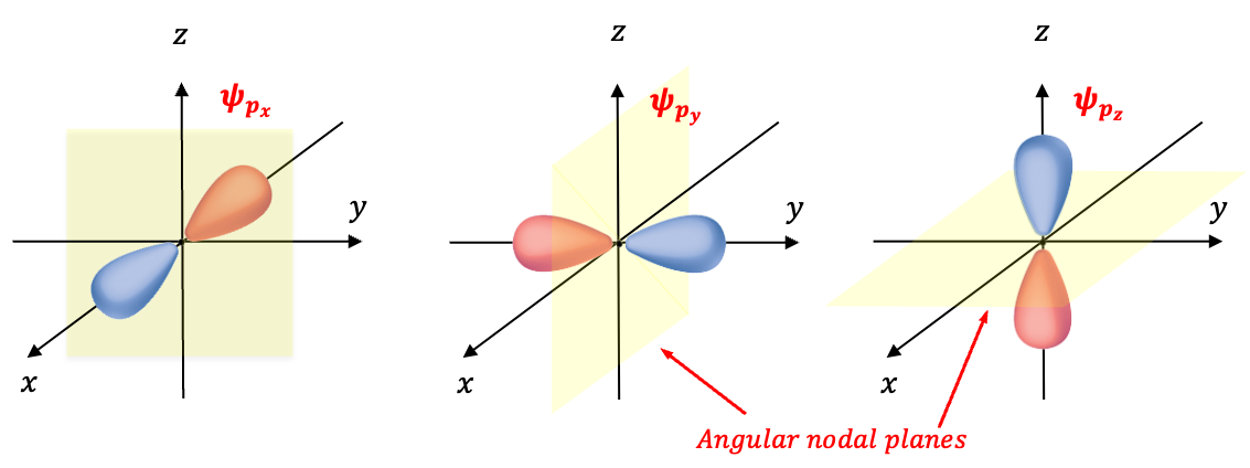
One-electron p-orbital wavefunctions can be expressed using the total wavefunction of a hydrogenic atom:

$\psi=R_{n,l}(r)Y_l^{\vert m_l\vert}(\theta,\phi)$

where

$R_{n,l}(r)=N_{n,l}\frac{1}{r}\biggr$\frac{r}{na_0}\biggr$^{l+1}e^{-\frac{r}{na_0}}L_{n-l-1}^{2l+1}\biggr$\frac{2r}{na_0}\biggr$$ , the radial wavefunction, is the radial component of $\psi$ .
$Y_l^{\vert m_l\vert}(\theta,\phi)=N_l^{\vert m_l\vert}P_l^{\vert m_l\vert}(cos\theta)e^{im_l\phi}$ , the spherical harmonics, is the angular component of $\psi$ .
$L_{n-l-1}^{2l+1}=\sum_{k=0}^{n-l-1}(-1)^k\frac{(n+l)!}{k!(k+2l+1)!(n-l-1-k)!}\biggr$\frac{2r}{na_0}\biggr$^k$ are the associated Laguerre polynomials.
$P_l^{\vert m_l\vert}(cos\theta)=\frac{1}{2^ll!}(1-cos^2\theta)^{\frac{\vert m_l\vert}{2}}\frac{d^{l+\vert m_l\vert}}{dcos\theta^{l+\vert m_l\vert}}(cos^2\theta-1)^l$ are the associated Legendre polynomials.
$N_{n,l}=\sqrt{\frac{(n-l-1)!}{2n(n+l)!}\frac{2^{2l+3}}{na_0}}$ is the normalisation constant of the radial wavefunction.
$N_l^{\vert m_l\vert}=\frac{1}{\sqrt{2\pi}}\biggr\[\frac{2l+1}{2}\frac{(l-\vert m_l\vert)!}{(l+\vert m_l\vert)!}\biggr\]^{\frac{1}{2}}$ is the normalisation constant of the spherical harmonics.
$n$ is the principal quantum number, where $n=1,2,\cdots$
$l$ is the orbital angular momentum quantum number (also known as azimuthal quantum number), where $l=0,1,2,\cdots$ and $l\leq n-1$ .
$m_l$ is the magnetic quantum number, where $-l\leq m_l\leq l$ .

The principal quantum number, $n$ , is also called a shell. Since $-1\leq m_l\leq 1$ when $l=1$ , there are three p-orbitals that are characterised by the set of quantum numbers $\{n,l,m_l\}$ of $\{n,1,0\}$ , $\{n,1,1\}$ and $\{n,1,-1\}$ in each shell for $n\geq 2$ . Each of the three p-orbitals has an angular node. Consider the set $\{2,1,0\}$ . Substituting these values into the explicit formula for $R_{n,l}(r)Y_l^{\vert m_l\vert}(\theta,\phi)$ yields:

$R_{2,1}(r)Y_1^{0}(\theta,\phi)=rcos\theta f(r)$

where $f(r)=\frac{1}{4\sqrt{2\pi}}\sqrt{\biggr$\frac{1}{a_0}\biggr$^5}e^{-\frac{r}{2a_0}}$ .

Converting from spherical coordinates to Cartesian coordinates, where $z=rcos\theta$ , gives

$\psi_{2p_z}=zf(r)\;\;\;\;\;\;\;\;474$

Eq474 is known as the $2p_z$ orbital. When $z=0$ , the wavefunction is zero everywhere in the $xy$ -plane, which is known as the nodal plane.

For the sets $\{2,1,1\}$ and $\{2,1,-1\}$ , we have ${\psi_{p_1}=\frac{1}{8\sqrt{\pi}}\sqrt{\biggr$\frac{1}{a_0}\biggr$^5}re^{-\frac{r}{2a_0}}(1-cos^2\theta)^{\frac{1}{2}}e^{i\phi}}$ and ${\psi_{p_{-1}}=\frac{1}{8\sqrt{\pi}}\sqrt{\biggr$\frac{1}{a_0}\biggr$^5}re^{-\frac{r}{2a_0}}(1-cos^2\theta)^{\frac{1}{2}}e^{-i\phi}}$ , respectively. These two wavefunctions include the factor $e^{\pm i\phi}$ , which may complicate calculations when they undergo symmetry operations. Therefore, we take linear combinations of these wavefunctions to form simpler wavefunctions. The first linear combination is ${\psi_{p_1}+\psi_{p_{-1}}=rsin\theta\cos\phi\frac{1}{4\sqrt{\pi}}\sqrt{\biggr$\frac{1}{a_0}\biggr$^5}e^{-\frac{r}{2a_0}}}$ , which normalises to ${rsin\theta\cos\phi\frac{1}{4\sqrt{2\pi}}\sqrt{\biggr$\frac{1}{a_0}\biggr$^5}e^{-\frac{r}{2a_0}}}$ , or equivalently in Cartesian coordinates:

$\psi_{2p_x}=xf(r)\;\;\;\;\;\;\;\;475$

since $x=rsin\theta cos\phi$ .

The second normalised linear combination is ${\psi_{p_1}-\psi_{p_{-1}}=rsin\theta\sin\phi\frac{1}{4\sqrt{2\pi}}\sqrt{\biggr$\frac{1}{a_0}\biggr$^5}e^{-\frac{r}{2a_0}}}$ , or equivalently,

$\psi_{2p_y}=yf(r)\;\;\;\;\;\;\;\;476$

since $y=rsin\theta sin\phi$ .

$\psi_{2p_x}$ and $\psi_{2p_y}$ , like $\psi_{2p_z}$ , each have an angular node.

Question

If ${\psi_{p_1}}$ and ${\psi_{p_{-1}}}$ are already normalised, why do we need to normalise a linear combination of them? How do we normalise a linear combination of ${\psi_{p_1}}$ and ${\psi_{p_{-1}}}$ ?

Answer

When forming a linear combination of normalised wavefunctions, the result is not necessarily normalised. Consider a general linear combination $\varphi=a\phi_1+b\phi_2$ , where $a$ and $b$ are coefficients. The normalisation condition for $\varphi$ requires that $\int\vert\varphi\vert^2d\tau=1$ , where $d\tau$ represents the volume element in spherical coordinates. Expanding $\int\vert a\phi_1+b\phi_2\vert^2d\tau=1$ and noting that $\phi_1$ and $\phi_2$ are orthonormal, we have $\vert a\vert^2+\vert b\vert^2=1$ . If $\vert a\vert^2+\vert b\vert^2\neq 1$ , which is the case for the two linear combinations of ${\psi_{p_1}}$ and ${\psi_{p_{-1}}}$ , $\varphi$ will not be normalised.

To normalise ${\psi_{p_1}-\psi_{p_{-1}}}$ , we have ${N^2\int\vert\psi_{p_1}-\psi_{p_{-1}}\vert^2d\tau=1}$ or

$-N^2\frac{1}{16\pi}\biggr$\frac{1}{a_0}\biggr$^5\int_0^{\infty}\int_0^{\pi}\int_0^{2\pi}r^2sin^2\theta sin^2\phi e^{-\frac{r}{a_0}}r^2drsin\theta d\theta d\phi=1$