Advanced Chemistry - Mono Mole

February 7, 2023February 1, 2026

Polytropic processes

A polytropic process is described by the formula $pV^n=c$ , where $n\in\mathbb{R}_{\geq 0}$ . The table below shows the association of different pV curves for ideal gases with the corresponding thermodynamic processes:

Question

Why is the projection (the curve obtained by representing the process in $(p,V,T)$ space on the $p-V$ plane ) an adiabat when $n=\frac{C_p}{C_V}$ and why is $V$ a constant when $n=\infty$ ?

Answer

From eq44 and eq46, $dU=C_VdT$ and $dH=C_pdT$ for an ideal gas. For adiabatic processes, $dU=w=-pdV$ and hence, $C_VdT=-pdV$ . Furthermore, $H=U+PV\;\;\Rightarrow\;\;dH=dU+pdV+Vdp$ . Since $dU+pdV=0$ , $dH=Vdp\;\;\Rightarrow\;\;C_pdT=Vdp$ . So,

$\frac{C_p}{C_V}=-\frac{Vdp}{pdV}\;\;\Rightarrow\;\;\frac{C_p}{C_V}\int\frac{dV}{V}=-\int\frac{dp}{p}$
$\Rightarrow\;\;\frac{C_p}{C_V}(lnV+c_1)=-(lnp+c_2)$

which rearranges to $pV^{\frac{C_p}{C_V}}=c_3$ , where $c_3=e^{-c_2-\frac{C_p}{C_V}c_1}$ .

For the second why, $pV^n=c\;\;\Rightarrow\;\;V=\left(\frac{c}{p}\right)^{\frac{1}{n}}$ . If $n\rightarrow\infty$ , $V\rightarrow 1$ .

Previous article: Line integral

Next article: Second law of thermodynamics (overview)

Content page of chemical thermodynamics

Content page of advanced chemistry

Main content page

February 7, 2023September 26, 2024

Line integral

A line integral is the integral of a multi-variable function along a curve. Line integrals can be categorised into scalar line integrals and vector line integrals. They are usually evaluated using parametric equations, which are then reduced to one or more scalar integrals.

Scalar line integrals

Let’s begin with scalar line integrals. A scalar function of two variables $f(x,y)$ is represented geometrically by a surface on a three-dimensional graph (see diagram above). Consider two points, A and B, on the surface. There are infinite ways to move along the surface between these two points. For simplicity, we have indicated two of these infinite paths using the red and pink curves, which can be projected onto the xy plane for better visualisation (see diagram below).

Due to the many paths available between the two points, the integral of $f(x,y)$ between the points is not well defined. In other words, the integral is path-dependent. For a particular path, the integral of $f(x,y)$ along this path, which is specified by one of the curves on the $xy$ plane, is called a line integral.

Geometrically, the result is the area of the ‘curtain’ extending from that path, between $(x_1,y_1)$ and $(x_2,y_2)$ on the xy plane, to the curve on the surface (see diagram above), i.e.:

$\int_cfds$

where $c$ denotes ‘curve’, which is the specified path linking the two points on the xy plane, and $ds$ is the infinitesimal change in arc length along the curve.

Since the specific path $c$ is also a function of $x$ and $y$ , we convert $f(x,y)$ and $c$ into parametric equations consisting of a single parameter and carry out the integration analytically (see 3rd Q&A below for an example).

Question

What if the two points, A and B, are the same?

Answer

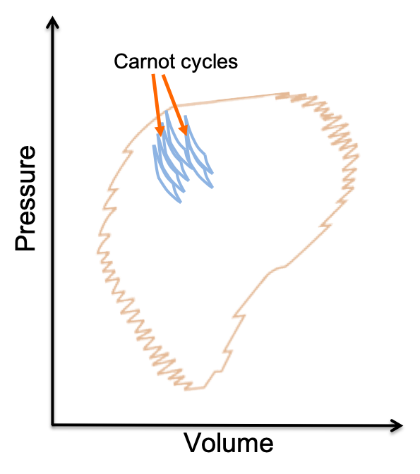
In the scenario where the two points are the same, the infinite paths from $(x_1,y_1)$ to $(x_1,y_1)$ are infinite loops. Similarly, integrating the function via different loops may give different results. Each line integral in this case is represented by:

$\oint_cfds$

where the circle on the integral sign denotes a loop or a cyclic process.

Vector line integrals

Let’s now look at vector line integrals, an example of which is the work done by a vector field (see diagram above). For instance, the work done by a variable force $\boldsymbol{\mathit{F}}$ on a charged particle moving along some path in an electric field is

$w=\int_c\boldsymbol{\mathit{F}}\cdot d\boldsymbol{s}\;\;\;\;\;\;\;\;(92)$

As mentioned in the opening paragraph, such a line integral is evaluated by converting it into one or more scalar integrals. We write $\boldsymbol{\mathit{F}}$ and $d\boldsymbol{\mathit{s}}$ in terms of their two-dimensional Cartesian components:

$\int_c\boldsymbol{\mathit{F}}\cdot d\boldsymbol{s}=\int_c(F_x\boldsymbol{i}+F_y\boldsymbol{j})\cdot( dx\boldsymbol{i}+dy\boldsymbol{j})=\int_cF_xdx+\int_cF_ydy$

which can then be evaluated when $c$ is specified.

Question

What is the difference between a scalar field and a vector field?

Answer

A scalar field, expressed by a scalar function $f(x,y)$ , associates a scalar with each point in some region of space, while a vector field, expressed by a vector function $\boldsymbol{\mathit{F}}(x,y)$ associates a vector with each point.

Line integral with respect to coordinates

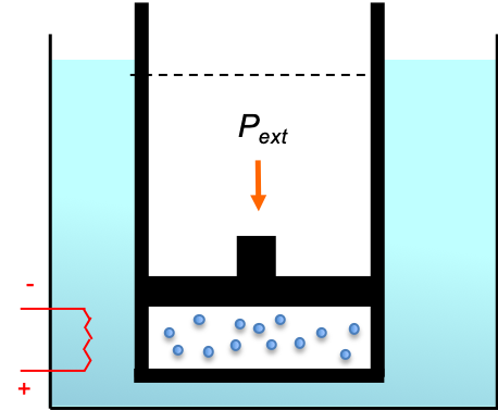
Line integrals can also be carried out with respect to one of the function variables instead of with respect to the arc length, e.g. the scalar integral $\int_cfdy$ . The geometric interpretation of $\int_cfdy$ is the projection of $\int_cfds$ on the $fy$ plane (see above diagram). An example of such a line integral is the work done on an ideal gas in a reversible process:

$w=-\int_cp(V,T)dV$

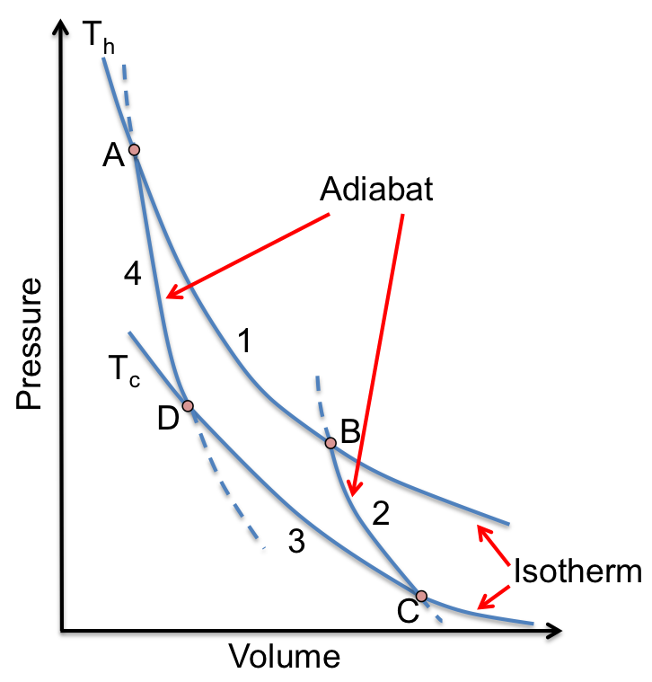
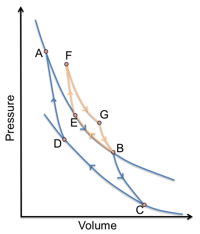
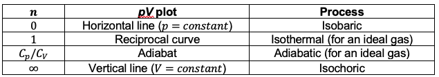
If the path of the above integral is defined by introducing a constraint, e.g. when $T=C$ , where $C$ is a constant, we get a plane that intersects with the surface at a particular contour (see diagram below). A single curve, an isothermal curve, is then projected on the $pV$ plane.

Consequently, the integral reduces to one involving a single variable:

$w=-\int_cp(V)dV=-nRT\int_{V_1}^{V_2}\frac{1}{V}dV$

Similarly, if the intersecting plane is $p=C$ or $V=C$ , the projection on the $pV$ plane is a horizontal line (isobaric process) or a vertical line (isochoric process) respectively.

Line integral of differential forms

Line integrals are sometimes written in differential form. Consider the work done by a vector field $\boldsymbol{\mathit{F}}(x,y)$ on a particle moving along some path $d\boldsymbol{s}(dx,dy)$ . We can write $\boldsymbol{\mathit{F}}$ and $d\boldsymbol{s}$ in terms of their components: $\boldsymbol{\mathit{F}}=F_x\boldsymbol{i}+F_y\boldsymbol{j}$ and $d\boldsymbol{s}=dx\boldsymbol{i}+dy\boldsymbol{j}$ . So, eq92 becomes

$w=\int_cdw=\int_c(F_x\boldsymbol{i}+F_y\boldsymbol{j}\cdot (dx\boldsymbol{i}+dy\boldsymbol{j})=\int_c\left(F_xdx+F_ydy\right)$

Compared to the general differential equation of two independent variables of the form $du=M(x,y)dx+N(x,y)dy$ , the RHS of the third equality of the above equation is the line integral of a differential equation, which in this case is an inexact differential. In other words, $\int_c\left(F_xdx+F_ydy\right)=\int_cdu$ .

In the case of an exact differential $df$ , its line integral is equal to the difference in values of the function $f$ at the final point and at the starting point:

$\int_cdf=f(x_2,y_2)-f(x_1,y_1)=\Delta f\;\;\;\;\;\;\;\;(93)$

This is known as the fundamental theorem of line integral. We call such a function, whose output is independent of the path taken to reach it, a state function.

Question

How do we proof the fundamental theorem of line integral?

Answer

Consider a function $f(x,y)$ with an exact differential of the form $df=\frac{\partial f}{\partial x}dx+\frac{\partial f}{\partial y}dy$ or

$df=\nabla f\cdot d\boldsymbol{r}$

where $\nabla f=\left(\boldsymbol{i}\frac{\partial}{\partial x}+\boldsymbol{j}\frac{\partial}{\partial y}\right)f$ and $d\boldsymbol{r}=dx\boldsymbol{i}+dy\boldsymbol{j}$ .

To carry out the line integral between two points $A$ and $B$ , we convert the function into its parametric form, which is to let $x$ and $y$ be some function of $t$ , i.e. $f\left(x(t),y(t)\right)\equiv f(t)$ . Correspondingly, we have $\boldsymbol{r}=x(t)\boldsymbol{i}+y(t)\boldsymbol{j}$ and hence $\frac{d\boldsymbol{r}}{dt}=\frac{dx(t)}{dt}\boldsymbol{i}+\frac{dy(t)}{dt}\boldsymbol{j}$ . So,

$\int_cdf=\int_c\nabla f\cdot d\boldsymbol{r}=\int_c\left[\frac{\partial f}{\partial x(t)}\frac{dx(t)}{dt}dt+\frac{\partial f}{\partial y(t)}\frac{dy(t)}{dt}dt\right]$

$\int_cdf=\int_A^B\left[\frac{\partial f}{\partial x(t)}\frac{dx(t)}{dt}+\frac{\partial f}{\partial y(t)}\frac{dy(t)}{dt}\right]dt$

Using the definition of the chain rule for a multivariable function (see eq14b),

$\int_cdf=\int_A^B\frac{df}{dt}dt=f(B)-f(A)\equiv f\left(x(B),y(B)\right)-f\left(x(A),y(A)\right)=\Delta f$

Finally, we have shown in a previous article that the change in internal energy of a system $\Delta U$ is path-independent for a system containing a perfect gas. We will show in the article on entropy that $\Delta U$ is path-independent for any system. This makes $dU$ an exact differential and $U$ , a state function. Thus, we can write

$\int_cdU=U(x_2,y_2)-U(x_1,y_1)=\Delta U$

If the two points are the same, $(x_2,y_2)=(x_1,y_1)$ ,

$\oint_cdU=\Delta U=0\;\;\;\;\;\;\;\;(94)$

Therefore, the change in internal energy in a cyclic process is zero: $\oint_cdU=0$ . In general, the line integral of any exact differential involved in a cyclic process is zero.

Previous article: Applications of The Joule-Thomson effect

Next article: Polytropic processes