Hund’s rules

Hund’s rules, created by Friedrich Hund in 1927, consist of three principles used to identify the lowest energy term symbol of a given atomic configuration. They are:

  • The term symbol with the highest multiplicity represents state(s) with the lowest energy.

This is due to the spin correlation between spin angular momenta of electrons, where the expectation value of the distance between a pair of electrons in the triplet state is greater than the expectation value of the distance between a pair of electrons in the singlet state. Consequently, there is less electron-electron repulsion for the triplet state (higher multiplicity) than for the singlet state.

  • For a particular multiplicity, the term symbol with the highest L is lowest in energy.

This results from the Coulomb interaction between orbital angular momentum of a pair of electrons, where electrons orbiting in the same direction meet less often than when they are orbiting in opposite directions. This implies that \vert\boldsymbol{\mathit{r}}_i-\boldsymbol{\mathit{r}}_j\vert_{ave}(same)>\vert\boldsymbol{\mathit{r}}_i-\boldsymbol{\mathit{r}}_j\vert_{ave}(opposite). Since the individual angular momentum of each electron orbiting in the same direction adds vectorially to give a higher total angular momentum (and hence a higher value of the quantum number L) than electrons orbiting in opposite directions, the term symbol with the highest L is lowest in energy.

  • Generally, for a particular term describing an atom with a less than half-filled outermost subshell, the term symbol with the lowest J is lowest in energy. If the subshell is more than half-filled, the term symbol with the highest J is lowest in energy.

This is because the value of A in eq289, which is empirically evaluated, generally changes from positive to negative when the subshell is more than half-filled.


Question

What about a half-filled subshell?

Answer

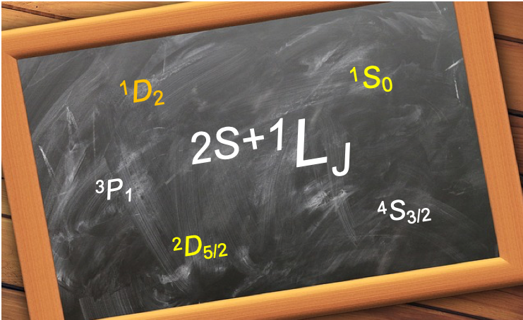
Examples of electron configuration of half-filled subshells are p3 and d5, with terms 4S and 6S respectively and corresponding levels of 4S3/2 and 6S5/2 respectively. Since the level of a half-filled subshell is described by only one term symbol, which always has the highest multiplicity of all microstates of the associated electron configuration, it is always lowest in energy. In other words, no rules are needed to determine the lowest energy term symbol of electron configurations like p3 and d5.


Since term symbols are based on Russell-Saunders coupling, where we assume that spin-spin coupling > orbit-orbit coupling > spin-orbit coupling, the three rules are applied in the above order (from rule 1 to rule 3) when we determine the lowest energy term symbol of a given configuration of an atom. The ground states of carbon and nitrogen are therefore 3P0 and 4S3/2 respectively.

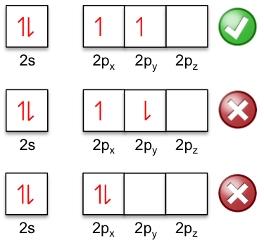
Hund’s rules are often stated as a single rule at introductory courses, with the rule being: electrons occupy the orbitals of a subshell singly and in parallel before pairing up. This statement is another way to state the first rule, which is the most dominant. Using the example of the n=2 shell of the ground state of carbon, the two electrons in the 2p orbitals are parallel because of the first rule.


Question

Why are the two electrons in the 2s orbital anti-parallel?

Answer

This is also a consequence of the first rule, where the spatial wavefunction associated with a triplet state is \psi=\frac{1}{\sqrt{2}}[\psi_a(r_1)\psi_b(r_2)-\psi_b(r_1)\psi_a(r_2)]. If r_1=r_2,  and \psi=0 and \int\vert\psi\vert^2d\tau=0, which implies that there is zero probability of finding the two parallel electrons at the same point.


Next article: The variational method
Previous article: Constructing atomic terms (coupled representation)
Content page of quantum mechanics
Content page of advanced chemistry
Main content page

Constructing atomic terms (coupled representation)

The construction of term symbols in the spin-orbit coupled representation (i.e. levels) is an extension of the procedure for deriving term symbols in the spin-orbit uncoupled representation (i.e. terms).


Russell-Saunders (LS) coupling

For the p2 configuration of the carbon atom, we have shown in the previous article that the terms are 1D, 3P and 1S with degeneracies (2L+1)(2S+1) of 5, 9 and 1 respectively. The total degeneracy of 15 corresponds to 15 microstates in the uncoupled representation, which are the basis states for the coupled representation. Since the total number of microstates describing a system is independent of the chosen representation, we have 15 coupled states after linearly combining the uncoupled basis states. The procedure to construct levels is to use the Clebsch-Gordan series, which describes the allow values of the total angular momentum number J for a given value of L and a given value of S, while ensuring that the total number of microstates (degeneracy) of each term (e.g. 3P) is equal to the total number of microstates of the associated levels (e.g. 3P2, 3P1, 3P0), i.e. (2L+1)(2S+1)=\sum_{allowed\: J}(2J+1)_{allowed\: J}.


Term

Degeneracy \boldsymbol{\mathit{J}}=\boldsymbol{\mathit{L}}+\boldsymbol{\mathit{S}} Level

Degeneracy

1D

5 2 = 2 + 0 1D2

5

3P

9

2 = 1 + 1 3P2 5
3P1

3

3P0

1
1S 1 0 = 0 + 0 1S0

1


For the p3 configuration of nitrogen, the terms are 4S, 2D, 2P and the levels are:

Term

Degeneracy \boldsymbol{\mathit{J}}=\boldsymbol{\mathit{L}}+\boldsymbol{\mathit{S}} Level Degeneracy
4S 4 3/2 = 0 + 3/2 4S3/2

4

2D

10 5/2 = 2 + 1/2 2D5/2 6
2D3/2

4

2P

6 3/2 = 1 + 1/2 2P3/2 4
2P1/2

2

You’ll notice that the degeneracies for both carbon and nitrogen are not fully lifted (i.e. each level may contain more than one state) when spin-orbit interactions are considered. Other effects, like an external magnetic field, are required to completed lift the degeneracy of an atom.


jj-coupling

In jj-coupling, each electron of the p2 configuration has and , which combine to give or . For each value of , there are  allowed values (see this article for details). Thus, each electron is described by the one-electron wavefunctions , , , , and , giving a total of six one-electron states.

According to the Pauli exclusion principle, no two electrons can can be described by the same set of quantum numbers. Therefore, two-electron wavefunctions like  are forbidden.

The 15 Pauli-allowed microstates can be grouped as follows:

For the group, the microstates with spanning from +2 to -2 form the term , with the remaining microstate with belonging to . Similarly, for the group, the microstates correspond to the terms and . Therefore, the jj-coupling term symbols for the p2 configuration are , , , and .


Next article: Hund’s rules
Previous article: Constructing atomic terms (uncoupled representation)
Content page of quantum mechanics
Content page of advanced chemistry
Main content page

Constructing atomic terms (uncoupled representation)

Consider the coupling of two electrons. From eq205, we have

\hat{J}=\hat{L}\otimes I+I\otimes\hat{S}

where \hat{L}=\hat{l}^{(1)}\otimes I+I\otimes\hat{l}^{(2)} and \hat{S}=\hat{s}^{(1)}\otimes I+I\otimes\hat{s}^{(2)}.

This implies that the state corresponding to \hat{L} is a coupled representation of \hat{l}^{(1)} and \hat{l}^{(2)} (orbit-orbit coupling), and that the state corresponding to \hat{S} is a coupled representation of \hat{s}^{(1)} and \hat{s}^{(2)} (spin-spin coupling). The overall state can be either a spin-orbit coupled representation \vert J,M_J,L,S\rangle, or a spin-orbit uncoupled representation \vert L,M_L,S,M_S\rangle. As mentioned in a previous article, if we neglect spin-orbit coupling, we can construct atomic terms using the uncoupled representation.

If the two electrons are in the same open subshell, they are called equivalent electrons. An example of such a system is the carbon atom. Even though carbon has six electrons, four of them are in closed shells with zero angular momentum and are therefore ignored when determining atomic terms.

The first step is to tabulate all possible microstates of p2 (arrangements of p2 electrons) that do not violate the Pauli exclusion principle:

Groups

\boldsymbol{\mathit{m}}_l \boldsymbol{\mathit{M}}_L \boldsymbol{\mathit{M}}_S

+1

0

-1

All up

u

u 1

1

u

u 0 1

u

u -1

1

All down d d 1

-1

d d 0

-1

d d -1 -1

One up, one down

ud

2 0

ud 0

0

ud -2

0

u d 1

0

u d 0

0

u d -1

0

d

u 1

0

d

u 0

0

d u -1

0

where u and d represent m_s=+\frac{1}{2} and m_s=-\frac{1}{2} respectively.

The above table is re-organised as:

\boldsymbol{\mathit{M}}_S

+1

0

-1

\boldsymbol{\mathit{M}}_L

+2

1

+1

1 2

1

0

1 3

1

-1

1 2

1

-2

1

where each green number represents the number of microstates corresponding to each (M_L,M_S) combination.

The only microstate with M_L=+2 and M_S=0 when expressed in the uncoupled representation of \vert L,M_L,S,M_S\rangle is \vert 2,2,0,0\rangle because L=M_{L,max}. It must belong to the term 1D, since 1D is when L=2 and S=0, with degenerate states of \vert 2,2,0,0\rangle, \vert 2,1,0,0\rangle, \vert 2,0,0,0\rangle, \vert 2,-1,0,0\rangle  and \vert 2,-2,0,0\rangle. For accounting purposes, we refresh the above table by removing these 5 states of 1D, giving:

\boldsymbol{\mathit{M}}_S

+1

0

-1

\boldsymbol{\mathit{M}}_L

+2

+1

1 1

1

0

1 2

1

-1

1 1

1

-2

Similarly, the only state with M_L=+1,M_S=+1 must be one of the 9 degenerate states of 3P. Again, we refresh the above table by removing these 9 states of 3P, leaving behind one state (M_L=0,M_S=0), which corresponds to the term 1S. Therefore, the atomic terms for the p2 configuration of carbon are 1D, 3P and 1S.


Question

Why are the 9 degenerate states of 3P, combinations of M_L=+1,0,-1 and M_S=+1,0,-1?

Answer

Recall that states with same L and same S have the same energy and are grouped into a term. For the term 3P, L=1 and S=1 with degeneracy 9 (3P2 has 5, 3P1 has 3 and 3P0 has 1). For S=1, we have three spin-coupled basis vectors associated with the quantum numbers M_S=+1,0,-1 (formed by the coupling of s_1 and s_2). For L=1, we have another three orbit-coupled basis vectors associated with the quantum numbers M_L=+1,0,-1 (formed by the coupling of l_1 and l_2). The total uncoupled microstates \vert L,M_L,S,M_S\rangle are the number of ways to form Kronecker products of basis vectors from the two vector spaces and hence combinations of M_L=+1,0,-1M_L=+1,0,-1 and M_S=+1,0,-1.


For the configuration 1s22s22p3, e.g. nitrogen, we have

Groups \boldsymbol{\mathit{m}}_l \boldsymbol{\mathit{M}}_L \boldsymbol{\mathit{M}}_S
+1 0 -1
All up u u u 0 3/2
All down d d d 0 -3/2
One up two down ud d 2 -1/2
ud d 1 -1/2
d ud 1 -1/2
ud d -1 -1/2
d ud -1 -1/2
d ud -2 -1/2
u d d 0 -1/2
d u d 0 -1/2
d d u 0 -1/2
Two up one down ud u 2 1/2
ud u 1 1/2
u ud 1 1/2
ud u -1 1/2
u ud -1 1/2
u ud -2 1/2
u u d 0 1/2
u d u 0 1/2
d u u 0 1/2

We can re-organise the above table as:

\boldsymbol{\mathit{M}}_S
+3/2 1/2 -1/2 -3/2
\boldsymbol{\mathit{M}}_L +2 1 1
+1 2 2
0 1 3 3 1
-1 2 2
-2 1 1

The only state with M_L=0,M_S=+3/2 must be one of the 4 degenerate states of 4S. For accounting purposes, we re-tabulate the above table by removing these 4 states of 4S, giving:

\boldsymbol{\mathit{M}}_S
+3/2 1/2 -1/2 -3/2
\boldsymbol{\mathit{M}}_L +2 1 1
+1 2 2
0 2 2
-1 2 2
-2 1 1

A good guess for the next term is 2D with a degeneracy of 10, because we are left with states of M_S=\pm1/2, spanning M_L from +2 to -2. The remaining states are:

\boldsymbol{\mathit{M}}_S
+3/2 1/2 -1/2 -3/2
\boldsymbol{\mathit{M}}_L +2
+1 1 1
0 1 1
-1 1 1
-2

which obviously belong to the term 2P.

Therefore, the terms for the configuration of nitrogen are 4S, 2D, 2P.

For a system with non-equivalent electrons (electrons in different subshells) in open shells, the way to construct atomic terms is similar to a system with equivalent electrons, except that we do not have to apply the Pauli exclusion principle in the construction process. The easiest method of construction is to use the Clebsch-Gordan series by coupling the l_i values to find out the possible L values, and then coupling the s_i values to give the possible S values, and finally combining the possible L and S values to produce the atomic terms. For example, the terms for the 2p13p1 system are 3D, 1D, 3P, 1P, 3S and 1S.


Next article: Constructing atomic terms (coupled representation)
Previous article: Term symbols
Content page of quantum mechanics
Content page of advanced chemistry
Main content page

Term symbols (quantum mechanics)

Term symbols are notations representing energy levels of a particular electron configuration of a chemical species.


Atomic term symbols

For light atoms, an atomic term symbol is based on Russell Saunders (LS) coupling and can be expressed either as:

^{2S+1}L\; \; \; \; \; \; \; \; 291

or

^{2S+1}L_J\; \; \; \; \; \; \; \; 292

where 2S+1 is called the multiplicity of the term symbol, S is the total spin angular momentum quantum number, L is the total orbital angular momentum quantum number and J is the total angular momentum quantum number.

Each value of L is further assigned a letter:

L 0 1 2 3 4 5 6 7 8
Letter S P D F G H I K L

Energy levels denoted by eq291 ignore spin-orbit coupling and are called terms, while those denoted by eq292 take into account spin-orbit coupling and are known as levels. Eq291 implies that for a particular electron configuration of an atom, states with the same set of angular momentum quantum numbers L and S have the same energy. We have shown in an earlier article how this is possible. When spin-orbit coupling effects are considered, degenerate states corresponding to a term are split into multiple levels. From eq248 and eq289, energy levels of a particular electron configuration of an atom are dependent on the quantum numbers J, L and S.


Question

Write the term symbols for i) the ground state of the hydrogen atom, and ii) the excited state of the hydrogen atom with the electron in the 2p orbital.

Answer

For the ground state of hydrogen, where S=s=\frac{1}{2} and L=0\equiv S, it is denoted by ^2S_{\frac{1}{2}}. For the excited state, the electron can be in any of the three degenerate 2p orbitals with either an up spin or a down spin. We would therefore expect two term symbols. The first symbol is ^2P_{\frac{3}{2}}, while the second symbol is obtained using the Clebsch-Gordan series of eq219 and is ^2P_{\frac{1}{2}}.


Question

Why is a term symbol not described by the principal quantum number ?

Answer

Term symbols focus on the variation of energy resulting from the arrangement and interaction of electrons in subshells. These arrangements, known as microstates, depend on whether the electrons are equivalent (belonging to the same subshell) or non-equivalent (belonging to different subshells). For example, the electrons in the configuration are equivalent, while those in are not. The term symbols for and are and respectively. Although the term symbols for and  are the same, the energies of the terms for , which are determined spectroscopically, differ from those for . Therefore, while the energy associated with does influence the overall energy of the electron within the atom, it doesn’t directly contribute to the variation in energies of electrons within the subshells.


As we move down the periodic table to heavier elements, such as lead or the actinides, spin-orbit interactions become so strong that  and are no longer good quantum numbers. In these cases, we switch to jj-coupling, where the individual and couple to form a for each electron, and the total angular momentum of the atom is obtained by vectorially adding these: . The corresponding atomic term symbol is:

For example, the term symbols for the configuration (see this article for details) are , , , and .

Even when jj-coupling is technically more accurate for heavy atoms, chemists often stick to the LS notation because it’s more intuitive for discussing symmetry and spectroscopy.

Molecular term symbols

Molecular term symbols are denoted by irreducible representations of the molecule’s point group because eigenstates of the molecular Hamiltonian transform according to irreducible representations of that group.

In linear molecules, the spherically symmetric electric field experienced by an electron in an atom is replaced by a cylindrically symmetric field about the molecular axis. As a result of this cylindrical symmetry, electrons experience a non-zero torque that causes their orbital angular momentum to precess about the molecular axis (taken as the -axis).


Question

Explain why a non-zero torque is generated on the electrons.

Answer

Classically, electrons are constantly moving around the nucleus of an atom. In an isolated atom, the potential is spherically symmetric, so the force on an electron is purely radial: . As a result, the torque vanishes.

In a linear molecule, however, the electronic potential is no longer spherically symmetric but cylindrically symmetric about the molecular axis. When an electron’s orbital motion is tilted relative to this axis, the force acting on the electron generally has components that are not parallel to . Consequently, , and a non-zero torque is generated on the electrons.


To explain the precessional motion, we show that the Hamiltonian is invariant under rotations about the -axis, but not the – and -axes. Consider the Hamiltonian of a diatomic molecule in which the electronic potential term is:

where , and are the position vectors of the electron, the first nucleus and the second nucleus respectively.

Using the Born-Oppenheimer approximation, the nuclear positions are fixed and a rotation operator acts only on the electronic coordinates. Let , and . Then and . Therefore, and hence is invariant under a rotation about the -axis ( doesn’t change), but not around the – and -axes (both and changes). It follows that , while and (see this article for details). Thus, only the projection of (denoted by ) along the molecular axis is a constant of motion.

The corresponding molecular term symbol for a linear molecule is:

where is the projection of the total electronic angular momentum onto the molecular axis and

Additional symmetry labels such as and (gerade and ungerade), as well as and , apply depending on the symmetry of the molecule. For example, the ground state of molecular oxygen, for which spin-orbit coupling is weak, is . If high-resolution spectroscopy is used, then we label the split states and .

For non-linear molecules, Mulliken symbols are used. For example, the ground state of water is .


Next article: Constructing atomic terms (uncoupled representation)
Previous article: russell saunders coupling
Content page of quantum mechanics
Content page of advanced chemistry
Main content page

Russell Saunders coupling

Russell Saunders coupling, or L-S coupling, is a method to derive the total angular momentum of a light multi-electron atom from its component angular momenta.

It assumes that spin-spin coupling > orbit-orbit coupling > spin-orbit coupling. This coupling scheme leads to the grouping of degenerate eigenstates into terms and levels, both of which correspond well with spectroscopic data of elements in the first three periods of the periodic table.

The total angular momentum \boldsymbol{\mathit{j}} of a 1-electron atom is defined as the vector sum \boldsymbol{\mathit{j}}=\boldsymbol{\mathit{l}}+\boldsymbol{\mathit{s}}, where \boldsymbol{\mathit{l}} and \boldsymbol{\mathit{s}} are the orbital angular momentum and spin angular momentum, respectively, of the electron in the atom. For an n-electron atom, Henry Russell and Frederick Saunders proposed that the total angular momentum \boldsymbol{\mathit{J}} of the atom is \boldsymbol{\mathit{J}}=\boldsymbol{\mathit{L}}+\boldsymbol{\mathit{S}}, where \boldsymbol{\mathit{L}}=\sum_{i=1}^n\boldsymbol{\mathit{l}}_i and \boldsymbol{\mathit{S}}=\sum_{i=1}^n\boldsymbol{\mathit{s}}_i. If we use a 2-electron atom as an example, the corresponding operator is:

\hat{J}=\hat{L}\otimes I+I\otimes\hat{S}\; \; \; \; \; \; \; \; 290

Since spin-spin coupling > orbit-orbit coupling > spin-orbit coupling, the spin angular momenta couple amongst themselves and the orbital angular momenta couple amongst themselves, before the total spin angular momentum couples with the total angular momentum. Hence, we have \hat{L}=\hat{l}^{(1)}\otimes I+I\otimes\hat{l}^{(2)} and \hat{S}=\hat{s}^{(1)}\otimes I+I\otimes\hat{s}^{(2)}. The eigenstates of \hat{L} are coupled representations of the basis vectors of \hat{l}^{(1)} and \hat{l}^{(2)}, while the eigenstates of \hat{S} are coupled representations of the basis vectors of \hat{s}^{(1)} and \hat{s}^{(2)}. The eigenstates of \hat{J} can either have the form of an uncoupled representation \vert L,M_L,S,M_S\rangle or a coupled representation \vert J,M_J,L,S\rangle. The uncoupled representation is used when spin-orbit coupling is very weak.

As we move down the periodic table to heavier elements, such as lead or the actinides, the spin-orbit interaction becomes so strong that and are no longer good quantum numbers. In these cases, we switch to  -coupling.


Next article: jj-coupling
Previous article: relativistic Many-electron Hamiltonian
Content page of quantum mechanics
Content page of advanced chemistry
Main content page

Relativistic many-electron Hamiltonian

The multi-electron Hamiltonian including the relativistic spin-orbit coupling term (but excluding other relativistic corrections) is

\hat{H}_R=\hat{H}_T+\hat{H}_{so}\; \; \; \; \; \; \; \; 283

where \hat{H}_T and \hat{H}_{so} are given by eq240 and eq261a, respectively.We shall now show that \hat{J}_z and \hat{J}^2 commute with \sum_{i=1}^n\boldsymbol{\mathit{S}}_i\cdot\boldsymbol{\mathit{L}}_i and therefore with \hat{H}_R. Assuming n=2,

\left[\hat{J}_z,\sum_{i=1}^2\boldsymbol{\mathit{S}}_i\cdot\boldsymbol{\mathit{L}}_i\right]=\left [\hat{L}_z^T+\hat{S}_z^T ,\sum_{i=1}^2\boldsymbol{\mathit{S}}_i\cdot\boldsymbol{\mathit{L}}_i\right ]=\left [\hat{L}_{1z}+\hat{L}_{2z}+\hat{S}_{1z}+\hat{S}_{2z} ,\sum_{i=1}^2\boldsymbol{\mathit{S}}_i\cdot\boldsymbol{\mathit{L}}_i\right ]

Expanding the RHS of the second equality of the above equation and using eq99, eq100, eq101, eq165, eq166 and eq167, \left[\hat{J}_z,\sum_{i=1}^2\boldsymbol{\mathit{S}}_i\cdot\boldsymbol{\mathit{L}}_i\right]=0. In general,

\left[\hat{J}_z,\sum_{i=1}^n\boldsymbol{\mathit{S}}_i\cdot\boldsymbol{\mathit{L}}_i\right]=0\; \; \; \; \; \; \; \; 284

Similarly,

\left[\hat{J}_x,\sum_{i=1}^n\boldsymbol{\mathit{S}}_i\cdot\boldsymbol{\mathit{L}}_i\right]=0\; \; \; \; \; and\; \; \; \; \;\left[\hat{J}_y,\sum_{i=1}^n\boldsymbol{\mathit{S}}_i\cdot\boldsymbol{\mathit{L}}_i\right]=0\; \; \; \; \; \; \; \; 285

Furthermore, [\hat{J}_z,\hat{H}_T]=[\hat{L}_z^T,\hat{H}_T]+[\hat{S}_z^T,\hat{H}_T]. Using eq243, [\hat{J}_z,\hat{H}_T]=0. Combining this with eq284,

\left[\hat{J}_z,\hat{H}_R\right]=0\; \; \; \; \; \; \; \; 286

Next,

\left[\hat{J}^2,\sum_{i=1}^2\boldsymbol{\mathit{S}}_i\cdot\boldsymbol{\mathit{L}}_i\right]=\left[\hat{J}_x^2,\sum_{i=1}^2\boldsymbol{\mathit{S}}_i\cdot\boldsymbol{\mathit{L}}_i\right]+\left[\hat{J}_y^2,\sum_{i=1}^2\boldsymbol{\mathit{S}}_i\cdot\boldsymbol{\mathit{L}}_i\right]+\left[\hat{J}_z^2,\sum_{i=1}^2\boldsymbol{\mathit{S}}_i\cdot\boldsymbol{\mathit{L}}_i\right]

Using the identity [\hat{A}\hat{B},\hat{C}]=[\hat{A},\hat{C}]\hat{B}+\hat{A}[\hat{B},\hat{C}] and substituting eq284 and eq285 in the above equation, \left[\hat{J}^2,\sum_{i=1}^2\boldsymbol{\mathit{S}}_i\cdot\boldsymbol{\mathit{L}}_i\right]=0. In general,

\left[\hat{J}^2,\sum_{i=1}^n\boldsymbol{\mathit{S}}_i\cdot\boldsymbol{\mathit{L}}_i\right]=0\; \; \; \; \; \; \; \; 287

Using eq244, eq245, \left[\hat{J}^2,\hat{H}_T\right]=\left[\hat{{L}^2}^T+\hat{{S}^2}^T+2\hat{\boldsymbol{\mathit{S}}}^T\cdot\hat{\boldsymbol{\mathit{L}}}^T,\hat{H}_T\right]=0. So,

\left[\hat{J}^2,\hat{H}_R\right]=0\; \; \; \; \; \; \; \; 288

Therefore, \hat{J}^2 and \hat{J}_z commute with \hat{H}_R. We have also shown in an earlier article that \hat{P}_{ij} commutes with \hat{J}^2, \hat{J}_z and \hat{H}_R. This implies that we can select a common complete set of eigenfunctions for \hat{J}^2, \hat{J}_z, \hat{P}_{ij} and \hat{H}_R. . Unlike the case of the hydrogen atom, \hat{{L}^2}^T and \hat{{S}^2}^T no longer commute with \hat{H}_{so} for a multi-electron atom (see eq182 and eq182a). Despite that, the quantum numbers J, L and S are used to characterise the states of elements in the first three periods of the periodic table, because spin-orbit coupling is weak for these atoms.

Similar to hydrogen, the eigenvalue equation of \hat{H}\psi=E\psi for a multi-electron atom is solved by treating \hat{H}_{so} as a perturbation if spin-orbit coupling is weak, with the unperturbed part of the eigenvalue equation solved using the Hartree-Fock method.


Question

Evaluate E_{so} using the first order perturbation theory.

Answer

For a multi-electron system, \hat{J}^2=\hat{L}^2+\hat{S}^2+2\hat{\boldsymbol{\mathit{L}}}\cdot\hat{\boldsymbol{\mathit{S}}}. So, \hat{\boldsymbol{\mathit{L}}}\cdot\hat{\boldsymbol{\mathit{S}}}=\frac{1}{2}\left ( \hat{J}^2-\hat{L}^2-\hat{S}^2\right ), which when substituted in E_{so}=\langle\psi\vert\xi(r)\hat{\boldsymbol{\mathit{L}}}\cdot\hat{\boldsymbol{\mathit{S}}}\vert\psi\rangle and using eq133, eq160 and eq205a, gives

E_{so}=A\frac{\hbar^2}{2}[J(J+1)-L(L+1)-S(S+1)]\; \; \; \; \; \; \; \; 289

where A=\langle\psi\vert\xi(r)\vert\psi\rangle=\biggl\langle\psi\left | \sum_{i=1}^n\frac{1}{2m_e^{\;2}c^2r_i}\frac{dV_i}{dr_i}\right |\psi\biggr\rangle.

A is evaluated empirically to be a constant for a given term.


Next article: Russell Saunders coupling
Previous article: relativistic one-electron Hamiltonian
Content page of quantum mechanics
Content page of advanced chemistry
Main content page

Relativistic one-electron Hamiltonian

The one-electron Hamiltonian including the relativistic spin-orbit coupling term (but excluding other relativistic corrections) adds the term in eq261 to eq45 to give:

\hat{H}=-\frac{\hbar^2}{2m_e}\nabla^2-\frac{Ze^2}{4\pi\varepsilon_0r}+\frac{1}{2m_e^{\;2}c^2r}\frac{dV}{dr}\hat{\boldsymbol{\mathit{L}}}\cdot\hat{\boldsymbol{\mathit{S}}}\; \; \; \; \; \; \; \; 282

or

\hat{H}=\frac{\hat{p}^2}{2m_e}-\frac{Ze^2}{4\pi\varepsilon_0r}+\frac{1}{2m_e^{\;2}c^2r}\frac{dV}{dr}\hat{\boldsymbol{\mathit{L}}}\cdot\hat{\boldsymbol{\mathit{S}}}

Since V=-\frac{Ze^2}{4\pi\varepsilon_0r}

\hat{H}=\hat{H}_0+\frac{1}{2m_e^{\;2}c^2}\frac{Ze^2}{4\pi\varepsilon_0r^3}\hat{\boldsymbol{\mathit{L}}}\cdot\hat{\boldsymbol{\mathit{S}}}

where \hat{H}_0=\frac{\hat{p}^2}{2m_e}-\frac{Ze^2}{4\pi\varepsilon_0r}.

From eq106 and eq107, we know that [\hat{L^2},\hat{H}_0]=0. We have also shown in an earlier article (Pauli matrices) that [\hat{L^2},\hat{\boldsymbol{\mathit{L}}}\cdot\hat{\boldsymbol{\mathit{S}}}]=0 and [\hat{S^2},\hat{\boldsymbol{\mathit{L}}}\cdot\hat{\boldsymbol{\mathit{S}}}]=0. Consequently, \left\[\hat{L^2},\frac{\hat{\boldsymbol{\mathit{L}}}\cdot\hat{\boldsymbol{\mathit{S}}}}{r^3}\right\]=0 and \left\[\hat{S^2},\frac{\hat{\boldsymbol{\mathit{L}}}\cdot\hat{\boldsymbol{\mathit{S}}}}{r^3}\right\]=0.


Question

Show that [\hat{J}^2,\hat{p}^2]=0, [\hat{J}^2,\frac{1}{r}]=0, [\hat{J^2},\hat{\boldsymbol{\mathit{L}}}\cdot\hat{\boldsymbol{\mathit{S}}}]=0 and [\hat{J}_z,\hat{\boldsymbol{\mathit{L}}}\cdot\hat{\boldsymbol{\mathit{S}}}]=0, where \hat{\boldsymbol{\mathit{J}}}=\hat{\boldsymbol{\mathit{L}}}+\hat{\boldsymbol{\mathit{S}}}.

Answer

Substituting \hat{J}^2=\boldsymbol{\mathit{J}}\cdot\boldsymbol{\mathit{J}}=\hat{L}^2+\hat{S}^2+2\boldsymbol{\mathit{L}}\cdot\boldsymbol{\mathit{S}}  in [\hat{J}^2,\hat{p}^2], expanding the expression and using eq104, we have [\hat{J}^2,\hat{p}^2]=0. Similarly, [\hat{J}^2,\frac{1}{r}]=0. Clearly, [\hat{J}^2,\boldsymbol{\mathit{L}}\cdot\boldsymbol{\mathit{S}}] =0. Finally, expanding the RHS of [\hat{J}_z,\boldsymbol{\mathit{L}}\cdot\boldsymbol{\mathit{S}}] =[\hat{J}_z,\hat{L}_x\hat{S}_x]+[\hat{J}_z,\hat{L}_y\hat{S}_y]+[\hat{J}_z,\hat{L}_z\hat{S}_z], noting that \hat{L}_i and \hat{S}_i act on different vector spaces and using eq100, eq101, eq166 and eq167, [\hat{J}_z,\boldsymbol{\mathit{L}}\cdot\boldsymbol{\mathit{S}}] =0.


Since \hat{L}^2, \hat{S}^2, \hat{J}^2 and \hat{J}_z all commute with \hat{H}, we can select a complete set of eigenfunctions in the form of \vert\hat{J}^2,\hat{J}_z,\hat{L}^2,\hat{S}^2\rangle for all operators. The eigenvalue equation of \hat{H}\psi=E\psi is solved by treating \hat{H}_{so}=\frac{1}{2m_e^{\;2}c^2}\frac{Ze^2}{4\pi\varepsilon_0r^3}\hat{\boldsymbol{\mathit{L}}}\cdot\hat{\boldsymbol{\mathit{S}}} as a perturbation.


Question

Evaluate E_{so} using the first order perturbation theory.

Answer

For a one-electron system, \hat{J}^2=\hat{L}^2+\hat{S}^2+2\boldsymbol{\mathit{L}}\cdot\boldsymbol{\mathit{S}}. So, \boldsymbol{\mathit{L}}\cdot\boldsymbol{\mathit{S}}=\frac{1}{2}(\hat{J}^2-\hat{L}^2-\hat{S}^2). Using this equation and eq133, eq160 and eq205a,

E_{so}=\langle\psi\vert\xi(r)\boldsymbol{\mathit{L}}\cdot\boldsymbol{\mathit{S}}\vert\psi\rangle=\langle\xi(r)\rangle\frac{\hbar^2}{2}[J(J+1)-L(L+1)-S(S+1)]

where \langle\xi(r)\rangle=\biggl\langle\psi\left | \frac{1}{2m_e^{\;2}c^2}\frac{ze^2}{4\pi\varepsilon_0r^3} \right |\psi\biggr\rangle.


Next article: Relativistic many-electron Hamiltonian
Previous article: Non-crossing rule
Content page of quantum mechanics
Content page of advanced chemistry
Main content page

Degenerate perturbation theory (an example)

Consider the eigenvalue equation of eq262 for a three-dimensional infinite cubical well, where

\hat{H}^{(0)}(x,y,z)=\left\{\begin{matrix} 0 & if\: 0<x<a,0<y<a,0<z<a\\ \infty & otherwise \end{matrix}\right.\; \; \; \; \; \; \; \; 277

\psi_{n_x,n_y,n_z}^{(0)}=\left ( \frac{2}{a} \right )^{\frac{3}{2}}sin\left ( \frac{n_x\pi}{a}x \right )sin\left ( \frac{n_y\pi}{a}y \right )sin\left ( \frac{n_z\pi}{a}z \right )\; \; \; \; \; \; \; \; 278

E_{n_x,n_y,n_z}^{(0)}=\frac{\pi^{2}\hbar^2}{2ma^2}(n_x^{\;2}+n_y^{\;2}+n_z^{\;2})\; \; \; \; \; \; \; \; 279

where n_x,n_y,n_z\in \mathbb{Z}^+.

From eq278, the ground state is \psi_{111}^{(0)}, while the first excited state is characterised by \psi_1=\psi_{112}^{(0)}, \psi_2=\psi_{121}^{(0)} and \psi_3=\psi_{211}^{(0)}. It is obvious, from eq279, that the first excited state is degenerate. Let’s assume that the potential in the well is perturbed such that first-order correction to \hat{H}^{(0)} is

\hat{H}^{(1)}=\left\{\begin{matrix} V_0,&if\: 0<x<\frac{a}{2},0<y<\frac{a}{2},0<z<a\\0& otherwise \end{matrix}\right.\; \; \; \; \; \; \; \; 280

We shall analyse the degenerate subspace of the first excited state. The first step is to compute the matrix elements W_{jl}=\langle\psi_{j,D1}^{(0)}\vert\hat{H}^{(1)}\vert\psi_{l,D1}^{(0)}\rangle and substitute them in eq274, with the assumption that \Psi_n^{(0)}=\alpha_1\psi_1+\alpha_2\psi_2+\alpha_3\psi_3:

\begin{pmatrix} \frac{V_0}{4} &0 &0 \\ 0 & \frac{V_0}{4} &\frac{16V_0}{9\pi^2} \\ 0 &\frac{16V_0}{9\pi^2} &\frac{V_0}{4} \end{pmatrix}\begin{pmatrix} \alpha_1\\\alpha_2 \\ \alpha_3 \end{pmatrix}=U_n^{(1)}\begin{pmatrix} \alpha_1\\\alpha_2 \\ \alpha_3 \end{pmatrix} \; \; \; \; \; \; \; \; 281

Finding the non-trivial solutions of the above linear homogeneous equation,

\begin{vmatrix} \frac{V_0}{4}-U_n^{(1)}&0 &0 \\ 0 & \frac{V_0}{4}-U_n^{(1)}&\frac{16V_0}{9\pi^2} \\ 0 &\frac{16V_0}{9\pi^2} &\frac{V_0}{4}-U_n^{(1)} \end{vmatrix}=0

\left ( \frac{V_0}{4}-U_n^{(1)}\right ) \left [\left ( \frac{V_0}{4}-U_n^{(1)}\right )^2-\frac{256V_0^2}{81\pi^4} \right ] =0

The roots are U_1^{(1)}=\frac{V_0}{4}, U_2^{(1)}= \frac{V_0}{4}+\frac{16V_0}{9\pi^2} and U_3^{(1)}= \frac{V_0}{4}-\frac{16V_0}{9\pi^2}, which means that the perturbation \hat{H}^{(1)} lifts the degeneracy of the unperturbed states. To find the exact eigenstates \Psi_n^{(0)}, we substitute the roots back in eq281. For the first root, we have

\begin{pmatrix} \frac{V_0}{4}\alpha_1\\\frac{V_0}{4}\alpha_2+ \frac{16V_0}{9\pi^2}\alpha_3\\ \frac{16V_0}{9\pi^2}\alpha_2+ \frac{V_0}{4}\alpha_3 \end{pmatrix}=\frac{V_0}{4}\begin{pmatrix} \alpha_1\\\alpha_2 \\ \alpha_3 \end{pmatrix}

Comparing both sides of the above equation, \alpha_1 can be any number but \alpha_2=0 and \alpha_3=0. So, the normalised wavefunction associated with U_1^{(1)} is \Psi_1^{(0)}=\psi_1. For the second root, we have

\begin{pmatrix} \frac{V_0}{4}\alpha_1\\\frac{V_0}{4}\alpha_2+ \frac{16V_0}{9\pi^2}\alpha_3\\ \frac{16V_0}{9\pi^2}\alpha_2+ \frac{V_0}{4}\alpha_3 \end{pmatrix}=\left ( \frac{V_0}{4}+\frac{16V_0}{9\pi^2}\right )\begin{pmatrix} \alpha_1\\\alpha_2 \\ \alpha_3 \end{pmatrix}

Comparing both sides, \alpha_1=0 since V_0\neq0, and \alpha_2=\alpha_3=1 (\alpha_2 and \alpha_3 are not equal to zero because that will result in \Psi_2^{(0)} being a zero eigenfunction). The normalised wavefunction associated with U_2^{(1)} is \Psi_2^{(0)}=\frac{1}{\sqrt{2}}(\psi_2+\psi_3). Similarly, for U_3^{(1)}, we have \Psi_3^{(0)}=\frac{1}{\sqrt{2}}(\psi_2-\psi_3).

Finally, by substituting \Psi_1^{(0)}, \Psi_2^{(0)} and \Psi_3^{(0)} in eq273, we find that they diagonalise \hat{H}^{(1)}. We call these linearly combined states that diagonalise \hat{H}^{(1)} “good” states.


Next article: Time-dependent perturbation theory
Previous article: Degenerate Perturbation theory
Content page of quantum mechanics
Content page of advanced chemistry
Main content page

Degenerate perturbation theory

The degenerate perturbation theory, an extension of the perturbation theory, is used to find an approximate solution to a quantum-mechanical problem involving non-perturbed states that are degenerate.

In the non-degenerate case, it is unambiguous that \Psi_n^{\;(0)}=\psi_n^{\;(0)}, i.e. \Psi_n^{\;(0)} is described by individual basis states \psi_n^{\;(0)}. However, for a set of degenerate orthonormal states \left \{\psi_{j,D1}^{\;(0)}\right \} (\small D1 denotes the same eigenvalue for all states in the set) of the unperturbed Hamiltonian \hat{H}^{(0)}, where \hat{H}^{(0)}\psi_{j}^{\;(0)}=E_{D1}^{\;(0)}\psi_{j}^{\;(0)}, \Psi_{n}^{\;(0)} can represent any linear combination of \left \{\psi_{j,D1}^{\;(0)}\right \} or the non-degenerate states \psi_{n}^{\;(0)}, where \psi_{n}^{\;(0)}\notin \left \{\psi_{j,D1}^{\;(0)}\right \}. If there are more than one set of degenerate states, each set with a distinct energy level, \Psi_{n}^{\;(0)} represents linear combinations of \left \{\psi_{j,D1}^{\;(0)}\right \}, linear combinations of \left \{\psi_{j,D2}^{\;(0)}\right \}, and so on, and individual states of \psi_{n}^{\;(0)}, where \psi_{n}^{\;(0)}\notin \left \{\psi_{j,DX}^{\;(0)}\right \}.

For each set of degenerate orthonormal states, e.g. \left \{\psi_{j,D1}^{\;(0)}\right \}, of the unperturbed Hamiltonian \hat{H}^{(0)}, the linear combination \small \Psi_{n}^{\;(0)}=\sum_{j=1}^{g}\alpha_j\psi_{j,D1}^{\;(0)} (where \small g is the degeneracy) is an eigenstate of \hat{H}^{(0)} with the same eigenvalue \small U_{n,D1}^{\;(0)}=E_{n,D1}^{\;(0)}:

\small \hat{H}^{(0)}\Psi_{n}^{\;(0)}=\sum_{j=1}^{g}\alpha_j\hat{H}^{(0)}\psi_{j,D1}^{\;(0)} =E_{n,D1}^{\;(0)}\sum_{j=1}^{g}\alpha_j\psi_{j,D1}^{\;(0)}=E_{n,D1}^{\;(0)}\Psi_{n}^{\;(0)} \; \; \; \; \; \; \; \; 271

Therefore, the derivation in the previous article branches off from eq267. While \small \Psi_{n}^{\;(0)} is no longer unambiguously described by individual basis states \small \psi_{n}^{\;(0)}, \small U_{n}^{\;(0)} is still \small E_{n}^{\;(0)}. So, eq267 becomes

\small \hat{H}^{(0)}\Psi_{n}^{\;(1)}+\hat{H}^{(1)}\Psi_{n}^{\;(0)}-E_{n}^{\;(0)}\Psi_{n}^{\;(1)}-U_{n}^{\;(1)}\Psi_{n}^{\;(0)}=0\; \; \; \; \; \; \; \; 272

Multiplying the above equation from the left by \small \Psi_{j}^{\;(0)*} and integrating,

( E_{j}^{\;(0)}-E_{n}^{\;(0)} )\langle\Psi_{j}^{\;(0)}\vert\Psi_{n}^{\;(1)}\rangle +\langle\Psi_{j}^{\;(0)}\vert\hat{H}^{(1)}\vert\Psi_{n}^{\;(0)}\rangle =0

When E_{j}^{\;(0)}=E_{n}^{\;(0)}, we have.

\langle\Psi_{j}^{\;(0)}\vert\hat{H}^{(1)}\vert\Psi_{n}^{\;(0)}\rangle =0\; \; \; \; \; \; \; \; 273

Since \langle\Psi_{j}^{\;(0)}\vert\hat{H}^{(1)}\vert\Psi_{n}^{\;(0)}\rangle represents the matrix elements of \hat{H}^{(1)}, eq273 implies that in the presence of degenerate states, the first-order perturbation theory only works if we can select appropriate wavefunctions that diagonalise \hat{H}^{(1)}.

Consider the case of just one set of degenerate orthonormal states \left \{ \psi_{l,D1}^{(0)} \right \} of the unperturbed Hamiltonian \hat{H}^{(0)}, with the other states of \hat{H}^{(0)} being non-degenerate. If we further analyse the subspace of \left \{ \psi_{l,D1}^{(0)} \right \}, we substitute \Psi_{n}^{\;(0)}=\sum_{l=1}^{g}\alpha_l\psi_{l,D1}^{\;(0)} in eq272 to give:

\hat{H}^{(0)}\Psi_{n}^{\;(1)}+\hat{H}^{(1)}\sum_{l=1}^{g}\alpha_l\psi_{l,D1}^{\;(0)}-E_{n,D1}^{(0)}\Psi_{n}^{\;(1)}-U_n^{(1)}\sum_{l=1}^{g}\alpha_l\psi_{l,D1}^{\;(0)}=0

Taking the inner product with \psi_{j,D1}^{\;(0)} and using eq36 on the first term,

\sum_{l=1}^gW_{jl}\alpha_l=U_n^{(1)}\alpha_l\; \; \; \; \; \; \; \; 274

where W_{jl}=\langle\psi_{j,D1}^{(0)}\vert\hat{H}^{(1)}\vert\psi_{l,D1}^{(0)}\rangle  are the matrix elements of \hat{H}^{(1)}.

Rewriting the eigenvalue equation of eq274 in matrix form,

\left [ \begin{pmatrix} W_{11} &W_{12} &\cdots &W_{1g} \\ W_{21} &W_{22} &\cdots &W_{2g} \\ \vdots &\vdots & \ddots &\vdots \\ W_{g1} & W_{g2}&\cdots &W_{gg} \end{pmatrix}-U_n^{(1)}I \right ]\begin{pmatrix} \alpha_1\\\alpha_2 \\ \vdots \\ \alpha_g \end{pmatrix}=0\; \; \; \; \; \; \; \; 275

where I is the g\times g identity matrix.

Eq275 is a linear homogeneous equation, which has non-trivial solutions if

\left | \begin{pmatrix} W_{11} &W_{12} &\cdots &W_{1g} \\ W_{21} &W_{22} &\cdots &W_{2g} \\ \vdots &\vdots & \ddots &\vdots \\ W_{g1} & W_{g2}&\cdots &W_{gg} \end{pmatrix}-U_n^{(1)}I \right |=0\; \; \; \; \; \; \; \; 276

Expanding the determinant (also known as a secular equation), we get the characteristic equation, which can be solved for the roots of U_n^{(1)}. Each of these roots is then substituted into eq274 to find the set of coefficients \alpha_l and hence, the exact eigenstates \Psi_n^{(0)}. If these exact eigenstates diagonalises \hat{H}^{(1)}, we refer to them as “good” states, which allow U_n^{(1)} to be calculated (see next article for an example).


Question

What is a linear homogeneous equation? Why does a linear homogeneous equation have non-trivial solutions if the determinant of the operator is zero?

Answer

A linear homogeneous equation is a matrix equation of the form A\boldsymbol{\mathit{X}}=0, where A is an n\times n matrix and \boldsymbol{\mathit{X}} is column vector. Let A be a 3\times3 matrix representing three position vectors  and \boldsymbol{\mathit{X}}=(x,y,z). We have

\begin{pmatrix} a_1 &a_2 &a_3 \\ b_1 & b_2 &b_3 \\ c_1 &c_2 &c_3 \end{pmatrix}\begin{pmatrix} x\\y \\ z \end{pmatrix}=\begin{pmatrix} a_1x+a_2y+a_3z\\b_1x+b_2y+b_3z \\ c_1x+c_2y+c_3z \end{pmatrix}=0

So, \boldsymbol{\mathit{a}}\cdot\boldsymbol{\mathit{X}}=0, \boldsymbol{\mathit{b}}\cdot\boldsymbol{\mathit{X}}=0 and \boldsymbol{\mathit{c}}\cdot\boldsymbol{\mathit{X}}=0. Now, a non-trivial solution of A\boldsymbol{\mathit{X}}=0 occurs when \boldsymbol{\mathit{X}}\neq0. Therefore, we require any non-zero position vector \boldsymbol{\mathit{X}} that is orthogonal to \boldsymbol{\mathit{a}},\boldsymbol{\mathit{b}},\boldsymbol{\mathit{c}}. This is fulfilled if the position vectors \boldsymbol{\mathit{a}},\boldsymbol{\mathit{b}},\boldsymbol{\mathit{c}} lie in a plane, which happens when the scalar triplet product \boldsymbol{\mathit{a}}\cdot(\boldsymbol{\mathit{b}}\times\boldsymbol{\mathit{c}}), which is equal to the volume of the parallelepiped spanned by \boldsymbol{\mathit{a}},\boldsymbol{\mathit{b}},\boldsymbol{\mathit{c}}, is zero. Since the scalar triple product is also equal to the determinant of A, i.e. \vert A\vert=\boldsymbol{\mathit{a}}\cdot(\boldsymbol{\mathit{b}}\times\boldsymbol{\mathit{c}}) (which can be easily proven by expanding both sides and showing that LHS equals to RHS), A\boldsymbol{\mathit{X}}=0 has non-trivial solutions if \vert A\vert=0.


Since there are multiple roots of U_n^{(1)}, the perturbation \hat{H}^{(1)} usually lifts the degeneracy of the unperturbed states. An example is the relativistic Hamiltonian’s spin-orbit coupling perturbation \hat{H}^{(1)}=\frac{1}{2m_e^{\;2}c^2r}\frac{dV}{dr}\hat{\boldsymbol{\mathit{L}}}\cdot\hat{\boldsymbol{\mathit{S}}}, which splits terms ^{2S+1}\textrm{\textit{L}} into levels ^{2S+1}\textrm{\textit{L}}_J. If there are equal roots, we would need to further analyse the problem with higher order perturbations to completely lift the degeneracy (as is the case when considering the Zeeman effect).


Question

Find the characteristic equation for the degenerate set \left \{ \psi_1^{(0)},\psi_2^{(0)} \right \}.

Answer

Eq276 becomes,

\left | \begin{pmatrix} W_{11} &W_{12} \\ W_{21} &W_{22} \end{pmatrix}-U_n^{(1)}I \right |=0

{U_n^{(1)}}^{2}-U_n^{(1)}(W_{11}+W_{22})+W_{11}W_{22}-W_{12}W_{21} =0


Next article: Degenerate perturbation theory (an example)
Previous article: Perturbation theory
Content page of quantum mechanics
Content page of advanced chemistry
Main content page

Perturbation theory

Perturbation theory is a method for finding an approximate solution to a problem by building on exact solutions of a simpler and related problem.

Consider the eigenvalue equation of

\hat{H}^{(0)}\psi_n^{\;(0)}=E_n^{\;(0)}\psi_n^{\;(0)}\; \; \; \; \; \; \; \; 262

where \hat{H}^{(0)} is the non-relativistic Hamiltonian, \psi_n^{\;(0)} is a complete set of orthonormal eigenfunctions that spans a Hilbert space, and E_n^{\;(0)} represents the exact eigenvalue solutions. We call \hat{H}^{(0)} and \psi_n^{\;(0)} the unperturbed Hamiltonian and unperturbed set of wavefunctions respectively.

If we extend the non-relativistic Hamiltonian to include certain interactions like spin-orbit coupling or a potential due to a ligand field, our eigenvalue equation in general is:

\hat{H}\Psi_n=U_n\Psi_n\; \; \; \; \; \; \; \; 263

where \hat{H} and \Psi_n are the perturbed Hamiltonian and perturbed set of wavefunctions respectively.

One common method of approximation is to write the new perturbed Hamiltonian as a power series in an arbitrary parameter \lambda:

\hat{H}=\hat{H}^{(0)}+\lambda\hat{H}^{(1)}+\lambda^{2}\hat{H}^{(2)}+\cdots\; \; \; \; \; \; \; \; 264

where \hat{H}^{(1)} and \hat{H}^{(2)} are the first-order and second-order corrections respectively to \hat{H}^{(0)}.

Similarly, the associated perturbed wavefunctions and energies of perturbed states are:

\Psi_n=\Psi_n^{\;(0)}+\lambda\Psi_n^{\;(1)}+\lambda^{2}\Psi_n^{\;(2)}+\cdots\; \; \; \; \; \; \; \; 265

U_n=U_n^{\;(0)}+\lambda U_n^{\;(1)}+\lambda^{2}U_n^{\;(2)}+\cdots\; \; \; \; \; \; \; \; 266

If we are satisfied with using just the first two terms in each of the power series of eq264, eq265 and eq266 for the approximation, we are dealing with what is known as the first-order perturbation theory. Substituting the first two terms in each of the three equations in eq263 and ignoring second-order quantities,

Since the parameters are arbitrary, they can be non-zero. If so, the only way to satisfy eq266 when U_n(\lambda)=0 is for U_n^{\;(0)}, U_n^{\;(1)}, U_n^{\;(2)} and so on to be zero. This implies that the powers of \lambda are independent variables. Consequently, the coefficients in eq266a must be zero:

\hat{H}^{(0)}\Psi_n^{\;(0)}-U_n^{\;(0)}\Psi_n^{\;(0)} =0

\hat{H}^{(0)}\Psi_n^{\;(1)}+\hat{H}^{(1)}\Psi_n^{\;(0)} -U_n^{\;(0)}\Psi_n^{\;(1)}-U_n^{\;(1)}\Psi_n^{\;(0)} =0\; \; \; \; \; \; \; \; 267

Substituting \Psi_n^{\;(0)}=\psi_n^{\;(0)} and U_n^{\;(0)}=E_n^{\;(0)} in eq267,

\hat{H}^{(0)}\Psi_n^{\;(1)}+\hat{H}^{(1)}\psi_n^{\;(0)} =E_n^{\;(0)}\Psi_n^{\;(1)}+U_n^{\;(1)}\psi_n^{\;(0)}\; \; \; \; \; \; \; \; 268

To find U_n^{\;(1)}, we multiply eq268 by \psi_n^{\;(0)*} and integrate; and use eq36 and the orthonormality of \psi_n^{\;(0)},

\langle\hat{H}^{(0)}\psi_n^{\;(0)}\vert\Psi_n^{\;(1)}\rangle+\langle\psi_n^{\;(0)}\vert\hat{H}^{(1)}\vert\psi_n^{\;(0)}\rangle =E_n^{\;(0)}\langle\psi_n^{\;(0)}\vert\Psi_n^{\;(1)}\rangle+U_n^{\;(1)}

U_n^{\;(1)}=\langle\psi_n^{\;(0)}\vert\hat{H}^{(1)}\vert\psi_n^{\;(0)}\rangle \; \; \; \; \; \; \; \; 269

Eq269 reveals that we can compute U_n^{\;(1)} using the first-order Hamiltonian and the complete set of wavefunctions of \hat{H}^{(0)}. However, the equation only works if all the wavefunctions are non-degenerate. To explain this limitation, we have to find the expression for \Psi_n^{\;(1)}. Since , the unperturbed wavefunction  can be fully characterised by the complete set \left \{ \psi_n^{\;(0)} \right \}. We therefore expand \Psi_n^{\;(1)}, which belongs to the same Hilbert space, as a linear combination of \left \{ \psi_n^{\;(0)} \right \}.


Question

Show that writing the linear combination as \Psi_n^{\;(1)}=\sum_{m\neq n}c_m\psi_m^{\;(0)} (i.e. \Psi_n^{\;(1)} has no \psi_n^{\;(0)} component) ensures that \Psi_n in eq263 is normalised with respect to the first order of \lambda.

Answer

When \Psi_n is normalised, \langle\Psi_n\vert\Psi_n\rangle=1. Substituting eq265 in this equation and expanding up to \lambda,

\langle\Psi_n\vert\Psi_n\rangle=1+\lambda\langle\Psi_n^{\;(1)}\vert\psi_n^{\;(0)}\rangle+\lambda\langle\psi_n^{\;(0)}\vert\Psi_n^{\;(1)}\rangle

If \Psi_n^{\;(1)} has no \psi_n^{\;(0)} component, i.e. \Psi_n^{\;(1)}\neq a\psi_n^{\;(0)}+b\psi_m^{\;(0)}+\cdots,

\langle\Psi_n\vert\Psi_n\rangle=1+0+0=1


Rearranging eq268 to \left ( \hat{H}^{(0)}-E_n^{\;(0)}\right )\Psi_n^{\;(1)}=\left ( U_n^{\;(1)}-\hat{H}^{(1)}\right )\psi_n^{\;(0)} and substituting \Psi_n^{\;(1)}=\sum_{m\neq n}c_m\psi_m^{\;(0)} in the equation,

\sum_{m\neq n}\left (E_m^{\;(0)}-E_n^{\;(0)}\right )c_m\psi_m^{\;(0)}=\left (U_n^{\;(1)}-\hat{H}^{(1)}\right )\psi_n^{\;(0)}

Multiplying the above equation by \psi_i^{\;(0)} and integrating,

\sum_{m\neq n}\left (E_m^{\;(0)}-E_n^{\;(0)}\right )c_m\langle\psi_i^{\;(0)}\vert\psi_m^{\;(0)}\rangle=U_n^{\;(1)}\langle\psi_i^{\;(0)}\vert\psi_n^{\;(0)}\rangle-\langle\psi_i^{\;(0)}\vert\hat{H}^{(1)}\vert\psi_n^{\;(0)}\rangle

If l=n, the above equation reduces to eq269. If l\neq n, only the term with \langle\psi_m^{\;(0)}\vert\psi_m^{\;(0)}\rangle survives, giving:

Substituting the above equation in \Psi_n^{\;(1)}=\sum_{m\neq n}c_m\psi_m^{\;(0)},

\Psi_n^{\;(1)}=\sum_{m\neq n}\frac{\langle\psi_m^{\;(0)}\vert\hat{H}^{(1)}\vert\psi_n^{\;(0)}\rangle}{E_n^{\;(0)}-E_m^{\;(0)}}\psi_m^{\;(0)}\; \; \; \; \; \; \; \; 270

The total wavefunction is \Psi_n=\Psi_n^{\;(0)}+\sum_{m\neq n}\frac{\langle\psi_m^{\;(0)}\vert\hat{H}^{(1)}\vert\psi_n^{\;(0)}\rangle}{E_n^{\;(0)}-E_m^{\;(0)}}\psi_m^{\;(0)}. If E_n^{\;(0)}=E_m^{\;(0)}, we have a problem. So, eq269 only works when all the wavefunctions are non-degenerate. If some of the wavefunctions are degenerate, we require another method called degenerate perturbation theory to calculate the eigenvalues.

To derive the second-order energy correction, we consider the following Schrodinger equation:

where we have used just a first-order correction to the Hamiltonian to simplify the calculations.

Collecting the powers of  and letting the coefficient be zero, we have

Multiplying the above equation by  and integrating over all space,

Using eq35, . So,

For ,

Since \Psi_n^{\;(1)}=\sum_{m\neq n}c_m\psi_m^{\;(0)}, we have . So,

It follows that the second-order energy depends on , which is a linear combination (mixing) of all other unperturbed eigenstates.

Substituting \Psi_n^{\;(1)}=\sum_{m\neq n}c_m\psi_m^{\;(0)} again and eq269a in the above equation, and using eq35 yields


Next article: Degenerate perturbation theory
Previous article: Spin-orbit coupling
Content page of quantum mechanics
Content page of advanced chemistry
Main content page
Mono Quiz