Hartree-Fock-Roothaan method

The Hartree-Fock-Roothaan method, an extension of the Hartree-Fock method, uses spin orbitals that are linear combinations of a set of basis wavefunctions .

Unlike the Hartree-Fock method, in which the parameters of the wavefunctions are varied, the best basis wavefunctions are chosen in the Hartree-Fock-Roothaan method and the coefficients are instead varied in an iterative process to determine the state of the system.

To derive the Hartree-Fock-Roothaan equations, we begin by substituting and in eq88, where we have relabelled and as and respectively, to give

where   .

Next we substitute , , and in eq92 to give

where   and .

Substituting eq152 and eq153 in eq94 gives

The constraint for the Lagrange method is found by substituting  and  in to give:

where .

Therefore, the Lagrangian is:

where  and are the undetermined multipliers.

As shown in the derivation of the canonical Hartree-Fock equations, we can select a set of coefficients and that diagonalises the Hermitian matrix with elements . The Lagrangian becomes

The total differential of the Lagrangian is

where .

Eq155 has the same form as eq12. If we can find a set of values of that renders the dependent variable terms of zero, we are left with the independent variable terms. Consequently, all the coefficients of are equal to zero and they form a set of equations that can be solved simultaneously. To simplify eq155, substitute eq154 in it to give

The next step involves the following:

    1. Renaming the dummy indices of the 5th and 6th terms by swapping i and j, and , and , and the dummy coordinates and .
    2. Noting that and .
    3. Noting that (see this article for explanation).
    4. Expanding each term of the equation and carrying out the partial differentiation.

We have,

Switching the dummy labels , and , , and the dummy coordinates and for the 1st term on the RHS of the above equation,

where the 1st term of the above equation is the complex conjugate of the 2nd term.

Since all coefficients of and are equal to zero, we have

where .

Similarly, the complex conjugate in eq156 gives:

Eq157 and eq158 are known as the Hartree-Fock-Roothaan equations.

Eq157 has non-trivial solutions if the determinant equals to zero. The computation process involves:

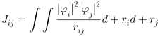
  1. Evaluating the integrals and either analytically or numerically using initial guess values of , and with basis wavefunctions where the parameters are fixed.
  2. Substituting the evaluated integrals in the characteristic equation and solving for , which is then used to obtain improved values of for the next iteration.
  3. Repeating steps 1 and 2 with the improved values of from the previous iteration until self-consistency is attained.
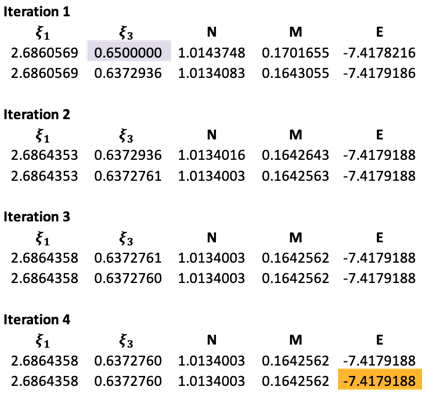
NEXT article: Solution of the Hartree-Fock-Roothaan equations for helium
Previous article: Atomic orbital energies
Content page of computational chemistry
Content page of advanced chemistry
Main content page

Antisymmetriser

An antisymmetriser is an operator that makes a wavefunction antisymmetric.

Consider a system of two-electrons, each of which is described by a spin-orbital.


Question

What is the difference between an orbital and a spin-orbital?

Answer

An orbital is a one-electron spatial wavefunction , i.e. a function that gives the best estimated energy eigenvalue of an electron when operated on by the Hamiltonian. For a given spatial orbital , we can form two spin-orbitals and , where and are spin functions. We say that the spatial orbital is doubly occupied by two electrons with the same energy. The abbreviated symbol of a spin-orbital is , where  represents the set of all 4 coordinates (3 spatial coordinates and 1 spin coordinate) associated with the electron.


The symmetric and antisymmetric forms of the total wavefunction of the system are and respectively. We have

where

      1.  .
      2.   is the identity operator.
      3. , like the exchange operator, swaps the labels of any two identical particles, i.e.

Eq59 implies that the antisymmetriser transforms the symmetric form of the wavefunction into a linear combination of states, each with a distinct permutation of spin-orbital labels. 

We can also expressed the antisymmetriser as , where an even (odd) numbered r represents an even (odd) number of times the labels are permutated. When the antisymmetriser acts on the wavefunction of an n-electron system, , we would expect the linear combination to have terms since there are  ways to permutate the labels. The antisymmetriser is therefore:

where N is the normalisation constant.

To evaluate N, we have

Due to the orthonormal property of , we find, after expanding the product of the linear combinations of and its complex conjugate, that the integrals result in terms of unity. Hence,

Substituting eq61 in eq60 yields:


Next article: Properties of the Antisymmetriser
Previous article: Analytical solution of the energy equation for He using the Hartree self-consistent field method
Content page of computational chemistry
Content page of advanced chemistry
Main content page

The expansion of \(\frac{1}{r_{ij}}\) (the reciprocal of the inter-electron distance)

The expansion of enables the Hartree equations to be solved analytically. Consider two electrons and  as depicted in the diagram below:

According to the law of cosines , which is equal to or

where .

Due to inter-electronic repulsion,  if is acute and hence , which implies that we can express eq35 as a binomial series, where  . Substituting  in the series, rearranging and displaying the terms of up to yields

Since the coefficients of the powers of are the Legendre polynomials , and that , we have

As mentioned in the previous article, is dependent on , , and (see diagram below). This implies that a function of like is a function of four angles. If we rotate the z-axis such that it lies on  , the vectors are expressed in a new coordinate system, where the new polar angle and azimuthal angle are   and  respectively. Consequently, we have , which is a simpler function to work with. We can also simplify the function in the original coordinate system by holding   and  as constants, resulting in a function of the variables and , or .

With reference to the new coordinate system, and its complex conjugate are eigenfunctions of with eigenvalue . For the original coordinate system, , and its complex conjugate are eigenfunctions of with the same eigenvalue .


Question

Show that the eigenvalue of   is in any three-dimensional coordinate system.

Answer

From eq108 and eq109, the quantum orbital angular momentum ladder operators for the original and new coordinate systems are and  respectively. The corresponding eigenfunctions of  and are and  respectively. Following the steps of determining the eigenvalues of and , we have and respectively.


Furthermore, the general solution of the eigenfunction of  is , where are the associated Legendre polynomials and are the coefficients of the basis polynomials in the linear combination. Therefore,

Question

Why is ?

Answer

For a particular value of , the linear combination is a sum of basis functions of a particular quantum angular momentum value . For example, when , we have a linear combination of the hydrogenic -orbital wavefunctions. Therefore, the eigenvalues of each term of the sum is always degenerate, which ensures that is an eigenfunction of .


To solve for , we multiply both sides of eq37 by the eigenfunction  and integrate over all space:

Due to the orthogonal property of associated Legendre polynomials, only the  term in the RHS expansion of the above equation survives,

From eq390, . Substituting this equation in the above equation and rearranging gives

To evaluate the integral in eq38, we expand the eigenfunction as a linear combination of basis functions in the new coordinate system:


Question

Why can we express in the original coordinate system as a linear combination of basis functions in the new coordinate system?

Answer

As mentioned earlier in the article,   and share the same set of eigenvalues. For a particular value of , is an eigenfunction of with a specific eigenvalue of , which is the same eigenvalue associated with for the same value of . In other words, , which implies that is invariant with respect to rotation of the coordinate system.


To solve for , multiply both sides of eq39 by , integrate over all space and repeat the steps in evaluating . We have

Next, eq39 must hold for the case of , with and . Expanding eq39,

From eq363a, , which is equal to zero if  and is equal to one if (because ), i.e.

So the only term that survives in eq41 is  and eq41 becomes

Substitute eq40, where and noting that , in eq43,

Substitute eq44 in eq38

Combining eq45, eq37 and eq36

Substitute in eq46, we have


Next article: Analytical solution of the energy equation for He using the Hartree self-consistent field method
Previous article: The angle between two vectors in spherical coordinates
Content page of computational chemistry
Content page of advanced chemistry
Main content page

Functional variation

Functional variation refers to the change in a functional’s output as a result of a small change in the functional’s input on a specified domain.


Question

What is a functional?

Answer

A functional is a function whose value depends on a function instead of an independent variable. For example, the expectation value of the Hamiltonian is a functional, where .


For a small variation in ,

where is a small arbitrary change in .

Since is small, , and

where .

If , we have or

which means that a small change in the functional’s input yields no change in the functional’s output. This implies a minimum energy according to the variational principle.


Next article: Proof of HArtree equations
Previous article: Lagrange method of undetermined multipliers
Content page of computational chemistry
Content page of advanced chemistry
Main content page

The angle between two vectors in spherical coordinates

The angle between two vectors in spherical coordinates is depicted in the diagram below:

We have

where and are the unit vectors of and , respectively.

Substituting eq182b (the unit vector in spherical coordinates) in eq33, noting that , and rearranging, gives


Next article: The expansion of \(\frac{1}{r_{ij}}\) (the reciprocal of the inter-electron distance)
Previous article: Numerical solution of the Hartree self-consistent field method for He
Content page of computational chemistry
Content page of advanced chemistry
Main content page

Numerical solution of the Hartree self-consistent field method for He

In this article, we shall calculate the ground state energy of a helium atom in one-dimension using an Excel spreadsheet. From eq5, the equations to be solved iteratively are:

The presence of multiple functions and variables in each of these equations requires us to devise a computation strategy, the first of which is to derive a trial wavefunction.


Question

Show that  is a reasonable wavefunction describing the helium ion.

Answer

The one-dimensional Schrodinger equation for the helium ion is , which can be written as


where , , and .

The general solutions of eq27 are of the form or . Let’s use , which is a modified form of a Slater-type orbital, where for the helium ion. Since , the normalisation constant N for y is . So, .


As the helium atom experiences an effective nuclear charge that is between that of a hydrogen atom () and a helium ion (), it can expressed by the trial wavefunction , which after normalisation is


Next, the pair of equations mentioned at the top of the article have two distinct wavefunctions, each representing one of the two electrons. To simplify our computation, we assume that the two electrons can be expressed by the same spatial wavefunction. This is known as the restricted case. To iteratively solve for the common wavefunction, we need to transform the two equations into a new pair of equations. Rearranging eq5 for helium in one-dimension, we have

where  and .

Substitute the definition of the 2nd derivative in eq29 and rearranging, we have

To prevent from being undefined when , we modify the Coulomb integral by adding a small constant C to the denominator. It is found that gives reasonable computation results. So,

The definition of the 1st derivative is
or:

Eq30 and eq31 are used in an iterative algorithm to find and . The procedure is as follows:

1) Set the boundary condition and . With reference to eq30, use eq28 as the initial guess wavefunction for the Coulomb integral. Let’s also assume an initial guess gradient of .

2) Let with intervals of (350 intervals in total). This implies that at .

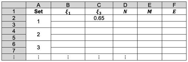
3) Use Simpson’s rule to integrate the Coulomb integral for all . An example of the excel table is shown below.


With reference to eq24, the formulae for cells C4, D4 and E4 are =(C2^2)*EXP(-2*1.5*C2)/(ABS(B4-C2)+0.5), =4*(D2^2)*EXP(-2*1.5*D2)/(ABS(B4-D2)+0.5) and =2*(E2^2)*EXP(-2*1.5*E2)/(ABS(B4-E2)+0.5) respectively. The formula for cell MP4 is =SUM(B4:MN4). Finally, the formula for cell MQ is 13.5*7/350/3*MP4, where 13.5 is the square of the normalisation constant of eq28. The formulae for the remaining cells within C4:MQ354 are populated accordingly.

4) The iterative table is formulated as follows:


The second row is for guess values and the error function. Rows 4 to 354 are for the algorithm. Cells MS2 and MV2 are the initial guess values of and b respectively. The formula for the normalisation constant in cell MU2 is =SQRT(((-MV2*2)^3)/2). Cell MS4 is obviously zero. The formula for cell MT4 is =MS2. With reference to eq29 and eq28, the formulae for cells MS5 and MT5 are, =MS4+MT4*(B5-B4) and =MT4+(MQ5-(2/B5)-MT2)*2*MS5*(B5-B4) respectively. The formulae for the remaining cells within MS4:MT354 are populated accordingly.

Next, we plot a graph using values in cells MS4:MS354 as vertical coordinates and B4:B354 as horizontal coordinates. By visually inspecting the graph, the value in cell MT2 is manually adjusted so that when . To optimise the values in cells MS2 and MV2, we include a trendline in the plot, where the formulae for cells MU4 and MU5 is zero and =MU2*B5*EXP(MV2*B5) respectively. The formulae for the remaining cells within MU4:MU354 are populated accordingly.

The error function formula in cell MW2 is {=SQRT(SUM((MS5:MS365-MU5:MU354)^2))}. The curly brackets {} are obtained by first typing the formula within {} in the cell and pressing CTRL+SHIFT+ENTER. Lastly, the Excel Solver application is use to optimise the values in cells MS2 and MV2, with the following settings:

Set objective: MW2
To: Min
By changing variable cells: MS2,MV2
Selecting a solving method: GRG Nonlinear

5) For the next set of iterations, repeat steps 3 and 4, where the guess values of MS2 and MV2 are the optimised values of the previous set of iterations. The value for MU is no longer the formula =SQRT(((-MV2*2)^3)/2) but the optimised normalisation constant of the previous set of iterations. Similarly, the values of and  used in the Coulomb integral in step 3 are no longer  and but the optimised values of MU2 and MV2 of the previous set of iterations.

6) The cycle continues until the values of , N and b are invariant up to five decimal points.

The results are summarized below:

To find  we use eq9, where

is taken from the 12th iteration set in the table above, while the double integral in eq32 is evaluated using form 2 of eq25. We being by computing the inner integral as per step 3, using and . Next, we apply the Simpson rule a second time for the outer integral. The Excel table is as follows:

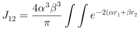
The formula for cell NA4 is =(4.838127^2)*(B4^2)*EXP(-1.802042*2*B4))*MQ4. With reference to form 2 of eq25, the formula in NC4 is =NA4*NB4*7/350/3, representing the double integral for . The formulae for the remaining cells within NA4:NB354 are populated accordingly. Summing NC4:NC354, we obtain the total value of the double integral of 1.1386946, which when substituted in eq32 together with gives . This theoretical value has a deviation of about 1.91% versus the experiment data of the ground state of helium.


Next article: The angle between two vectors in spherical coordinates
Previous article: Slater-type orbitals
Content page of computational chemistry
Content page of advanced chemistry
Main content page

Slater-type orbitals

Slater-type orbitals (STO) are mathematical functions that resemble hydrogenic wavefunctions. Introduced by John Slater in 1930, they are used as trial wavefunctions in computational chemistry to approximate the energies of molecular systems. The general form of an STO is:

where

N is a normalisation constant

n, and are quantum numbers

is the distance between an electron and the nucleus of an atom.

is the effective charge of the nucleus

represents the spherical harmonics

STOs with different n but the same and are not orthogonal to one another. When working with such STOs, the Gram-Schmidt process is used to convert the non-orthogonal orbitals to orthogonal ones.

Question

Show that the normalisation constant of a 1s orbital is .

Answer


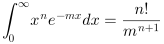
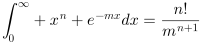
Using the identity (see this article for proof), we have .


Question

Using the identity , show that the 1s orbitals are orthogonal to each other but not orthogonal to the 2s orbital.

Answer


For the orbitals to be orthogonal to each other, either or needs to be zero, which is forbidden because the effective nuclear charge is not zero. Hence, the orbitals are not orthogonal to each other.


Next article: Numerical solution of the Hartree self-consistent method for He
Previous article: Simpson’s rule
Content page of computational chemistry
Content page of advanced chemistry
Main content page

Simpson’s rule

Simpson’s rule is a numerical method that uses quadratic functions to approximate definite integrals.

With reference to the diagram above, is the area under the cubic curve demarcated by two equal intervals, each of magnitude h. The area is estimated using 3 points on the quadratic function , where

Substituting , and into gives , and . Combining the last two equations gives . Substituting this equation and into eq23 yields

Similarly, if we consider the domain from h to h‘ (see above diagram),

Therefore, using 5 points on results in:

Extending the logic for n points on ,


where and .

This implies that there must be an even number of equal intervals for the rule to work, i.e. n must be odd.


Question

Evaluate

Answer

Substituting eq24 into the above equation yields:

So,

where (form 1)

or equivalently (form 2),

These integrals are useful for computing the numerical solution of the Hartree self-consistent field method for helium.


Next article: Slater-type orbitals
Previous article: Proof of the Hartree equations
Content page of computational chemistry
Content page of advanced chemistry
Main content page

Lagrange method of undetermined multipliers

The Lagrange method of undetermined multipliers is a technique for finding the maximum or minimum value of a function subject to one or more constraints.

Consider the function . The total differential of the function is

Since x and y are independent variables (see below diagram), the maximum value of the function occurs at the point where and , i.e.

In general, the extremum of a function with i-independent variables is at the point where all .

If we want to find the extremum of subject to a constraint, e.g. , we will realise that one of the variables, e.g. y, in is no longer independent. This is because we can substitute the constraint in the function to eliminate the dependent variable y and then let the 1st derivative of the function with respect to the remaining independent variable x be zero. However, this simple method of substitution becomes complicated when the problem involves more than two variables and more than one constraint.

In 1804, Joseph-Louis Lagrange devised another procedure to handle such problems. For the above example, the procedure involves transforming the constraint into the function , where . The total differential of g is

where and .

Since , and . This means that we can multiply throughout by a factor and add the result to (or subtract from) eq10 to obtain the total differential of a new function:

where .

The extremum of this function occurs when

If there is a , where , then it renders the dependent variable term , and we are left with the independent term . Solving the equations , and the constraint simultaneously, we can determine x, y and . This procedure is called the Lagrange method of undetermined multipliers. The factor is the multiplier, which is undetermined because it need not be solved to find the extremum of the function.

To evaluate the extremum of the n-independent variables function subject to m constraints, where , eq11 becomes

where .

If we can find a set of values of that renders all the m dependent variable terms zero, we have m equations of

leaving us with independent variable terms and equations of

This implies that each in eq12 can now vary arbitrarily. The values of all the variables and multipliers corresponding to the extremum are finally obtained by solving eq13, eq14 and all the constraint equations simultaneously. The Lagrange method of undetermined multipliers is used in the derivations of the Boltzmann distribution, the Hartree self-consistent field method, the Hartree-Fock method and the Hartree-Fock-Roothaan method.


Next article: Functional variation
Previous article: the hartree self-consistent field method
Content page of computational chemistry
Content page of advanced chemistry
Main content page

The Hartree self-consistent field method

The Hartree self-consistent field method is an iterative procedure that optimises an approximate wavefunction using the variational principle. Its goal is to estimate the eigenvalues of a modified form of the non-relativistic multi-electron Hamiltonian. This method was developed by the English scientist Douglas Hartree in 1927.

In an earlier article, we showed that the three dimensional Hamiltonian operator for an n-electron atom (excluding spin-orbit and other interactions) is:

where , and .

Our objective now is to solve eigenvalue equations for . The eigenvalue equation of the hydrogen atom has an exact solution (i.e. a solution represented by a formula). However, for an atom with more than one electron, the inter-electronic repulsion term poses a problem, which is a three-body problem that has no exact solution. Therefore, approximation methods are needed.

Firstly, we simplify the Hamiltonian by rewriting it in a system devised by Hartree called “atomic units” (abbreviated to a.u.), where ( is the Bohr radius, where ). For example, if the charge of a particle is 3.4 a.u., it is in S.I. units. Eq1 therefore becomes

with the eigenvalues of also in atomic units.

Secondly, we approximate the form of a multi-electron wavefunction. As hydrogenic wavefunctions have exact solutions, it is logical to express the multi-electron wavefunction as products of orthonormal one-electron spatial wavefunctions :

Thirdly, we utilise the variational principle, which states that the calculated energy is always greater than or equal to the ground state of any system. This implies that we can calculate an upper bound to of any system using a trial function . The closer the trial function is to the actual or best wavefunction of the system , the closer E will be to .

Using eq3 and eq2, we have

Simplifying the above equation and minimising E (see this article for proof), we obtain the following set of n ‘one-particle’ equations called the Hartree equations:

where .

Question

How do we interpret eq5?

Answer

Eq5 can be perceived as a set of n Schrodinger equations, each consisting of a modified one-electron non-relativistic Hamiltonian. Solving each of the n equations gives a minimised value of corresponding to the i-th electron.

To further explain the modified inter-electronic repulsion term, we refer to eq2. Focussing on electron 1, we have

We regard electrons 2, 3, …, n as being smeared out into a continuous and spherically symmetrical charge distribution through which electron 1 moves. For example, the interaction between electron 1 and electron 2 is

where is the charge density of (i.e. charge per unit volume) of electron 2.

Since , and , we have and hence . So,

The total potential energy between electron 1 and all other electrons is therefore


Since eq5 is the outcome of minimising eq4, subject to the constraints of the orthonormality of one-electron wavefunctions that make up the overall wavefunction of a system, any solution set of from eq5 is associated with a set of , each of which is also obtained from multiplying eq5 by and integrating over all space:

where and .

Summing all of eq6, we have

Since for the Coulomb term (see this article for explanation),

To establish the relation between E and , we rewrite eq4 as

where we have used the fact that is equivalent to (see this article for explanation).

Combining eq7 and eq8,

E is greater than the ground state of the system, except when the solution set is associated with the set of one-electron wavefunctions that best describes the ground state of the system, in which case E is the best estimate of . This best set of and the corresponding set of are found using the Hartree self-consistent field method, which involves the following steps:

  • Make guesses for all single-electron wavefunctions except for one, e.g. use trial functions for except . The corresponding equation to solve is:

Solving the above equation means finding and , which can only be done numerically because of the presence of unknown functions and variables (see this article for an example). The solutions are then the first approximations of and , which leads to a first improvement to eq3.

  • To further improve the wavefunction of eq3, we solve for and using

  • As per the previous step, the same trial functions for are employed together with the computed . The solutions are then the 1st approximation of and , and hence a further improvement to eq3.
  • Next, and derived from the previous two steps are used along with trial functions for to solve for and . The process is repeated until and are solved. The entire cycle is then repeated, i.e. step 1 is repeated using improved wavefunctions of to solve for an even better approximation of , and then followed by step 2 and step 3. This cyclical process stops when all and become invariant, which implies that the best approximation of eq3 for the particular system has been derived.
  • Finally, E is computed with eq9 using the derived and .

As the numerical method of calculating E is usually quite complex, an analytical method is often used. Such a method involves finding analytical expressions for all terms in eq8 using trial one-electron wavefunctions. As per the numerical method, guess values are used for the variables in all trial one-electron wavefunctions except one, e.g. . Eq8 is then minimised to obtain the solutions for E and . The process is repeated until E and all become invariant.

In conclusion, the Hartree self-consistent field method produces relatively accurate results when compared to experiment data for the ground state energy of a small atom like helium. However, it is less accurate for finding E of larger atoms, as it does not take into consideration exchange forces due to spin exchange interactions. A more accurate method, call the Hartree-Fock method is needed for such atoms.


Next article: Lagrange method of undetermined multipliers
Content page of computational chemistry
Content page of advanced chemistry
Main content page


Mono Quiz