The transition state theory provides a theoretical way to calculate the pre-exponential factor A and the activation energy Ea, and therefore the rate constant k of an elementary chemical reaction. This is in contrast with the Arrhenius equation, where A and Ea are obtained empirically. The theory is based on statistical thermodynamics and can be illustrated for a gas-phase bimolecular reaction using the following assumptions:
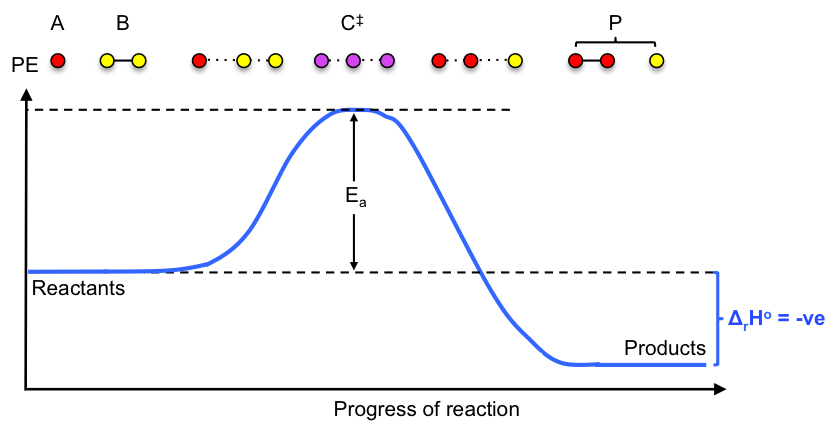
1) The reacting system, expressed as  , proceeds along an energy path that includes a point of highest potential energy called the saddle point, where a distinct species known as the activated complex
  is formed. The conversion of the activated complex to the product P can be seen as an asymmetric vibrational stretch:
2) A rapid pre-equilibrium is established between the activated complex and the reactants:  .
.
3) The rate of the reaction is attributed to the rate-determining step, which is the rate of conversion of the activated complex to the product: ![rate=k^{\ddagger}[C^{\ddagger}]](https://latex.codecogs.com/gif.latex?rate=k^{\ddagger}[C^{\ddagger}]) , where
, where  is proportional to the vibrational frequency
  of the activated complex.
The expression for the gas-phase rapid equilibrium from assumption 2 is:

which in terms of molar concentration is:
![K^{\ddagger}=\frac{p^o}{RT}\frac{[C^{\ddagger}]}{[A][B]}\; \; \; \; \; \; \; \; 1](https://latex.codecogs.com/gif.latex?K^{\ddagger}=\frac{p^o}{RT}\frac{[C^{\ddagger}]}{[A][B]}\;&space;\;&space;\;&space;\;&space;\;&space;\;&space;\;&space;\;&space;1)
Substituting eq1 into the rate equation , , yields:
![rate=k[A][B]\; \; \; \; \; \; \; where\; k=\frac{RT}{p^o}k^{\ddagger}K^{\ddagger}](https://latex.codecogs.com/gif.latex?rate=k[A][B]\;&space;\;&space;\;&space;\;&space;\;&space;\;&space;\;&space;where\;&space;k=\frac{RT}{p^o}k^{\ddagger}K^{\ddagger})

In general, the equilibrium constant, when written in terms of standard molar partition functions, is ![K=\left [ \prod _j\left ( \frac{q^o_{j,m}}{N_A} \right )^{v_j} \right ]e^{-\frac{\Delta_rE_0}{RT}}](https://latex.codecogs.com/gif.latex?K=\left&space;[&space;\prod&space;_j\left&space;(&space;\frac{q^o_{j,m}}{N_A}&space;\right&space;)^{v_j}&space;\right&space;]e^{-\frac{\Delta_rE_0}{RT}}) (see this article for derivation), where
(see this article for derivation), where  is the respective stoichiometric coefficient of the J-th species. For our bimolecular reaction,

where -E_0(A)-E_0(B)) .
.
The activated complex in our example is a linear molecule with N = 3 atoms and therefore has 3N – 5 = 4 modes of vibration (2 bending, 1 symmetric stretch and 1 asymmetric stretch). The standard molar partition function for the activated complex is the product of the partition functions of different modes of motion:  , which we can rewrite in the form:
  , where
  .
.
The standard molar partition function for the asymmetric vibration is  , where is the vibrational frequency that leads to the conversion of the activated complex to the product. Assuming
  ,
,  . Therefore,

Substituting eq3 into eq2 gives:

where 
Substituting eq4 into the rate constant equation  yields:

From assumption 3, is proportional to the vibrational frequency of the activated complex,

where  is the proportionality constant called the transmission coefficient, which accounts for the notion that not every oscillation of the activated complex leads to its conversion to the product.
Substituting eq6 into eq5 results in:

The standard Gibbs energy is  . By analogy, we define the standard Gibbs activation energy as
  , which we shall substitute into eq7 to give:


Question
Is the expression for standard Gibbs activation energy still valid when the equilibrium constant now excludes the factor  ?
?
Answer
It is an approximation that we make, which delivers an expression for the rate constant that is in good agreement with experimental values.
Eq7 and eq8 are different forms of the Eyring equation. Substituting eq8 in the definition of activation energy  and differentiating, noting that
  and
and  are standard states, which are temperature-independent, gives:

Substituting eq9 into eq8 yields:

Comparing eq10 and the Arrhenius equation, we have:

Repeating all the above steps for a gas-phase unimolecular reaction, we arrive at an activation energy of  instead of eq9. Therefore, the transition state theory predicts that the activation energy for a gas-phase elementary reaction is

where  for a unimolecular reaction and
  for a bimolecular reaction.