What is the formula of the titration curve of a diprotic acid versus a monoprotic strong base?
Consider a solution containing water, a diprotic acid of concentration Ca and a strong base of concentration Cb with the following equilibria:
\rightleftharpoons&space;H^+(aq)+OH^-(aq))
\rightleftharpoons&space;H^+(aq)+HA^-(aq)\;&space;\;&space;\;&space;\;&space;\;&space;\;&space;\;&space;\;&space;(13))
\rightleftharpoons&space;H^+(aq)+A^{2-}(aq)\;&space;\;&space;\;&space;\;&space;\;&space;\;&space;\;&space;\;&space;(14))
\rightleftharpoons&space;B^+(aq)+OH^-(aq))
With reference to charge balance of the above equilibria, the sum of the number of moles of cations H+ and B+ must equal to that of anions HA–, A2- and OH–. As the volume is of the solution is common to all ions,
![[H^+]+[B^+]=[OH^-]+[HA^-]+2[A^{2-}]\; \; \; \; \; \; \; \; (15)](https://latex.codecogs.com/gif.latex?[H^+]+[B^+]=[OH^-]+[HA^-]+2[A^{2-}]\;&space;\;&space;\;&space;\;&space;\;&space;\;&space;\;&space;\;&space;(15))
Read this article to understand how to arrive at eq15.
With reference to eq13 and eq14, at any point of the titration, the sum of the number of moles of H2A, HA– and A2– must equal to the number of moles of H2A if it were undissociated. As the change in volume of the solution is common to all ions,
![[H_2A]+[HA^-]+[A^{2-}]=\frac{C_aV_a}{V_a+V_b}\; \; \; \; \; \; \; \; (16)](https://latex.codecogs.com/gif.latex?[H_2A]+[HA^-]+[A^{2-}]=\frac{C_aV_a}{V_a+V_b}\;&space;\;&space;\;&space;\;&space;\;&space;\;&space;\;&space;\;&space;(16))
where Va and Vb are the volume of diprotic acid in the solution and the volume of strong monoprotic base in the solution respectively. The equilibrium constant equations of eq13 and that of eq14 are:
![[H_2A]=\frac{[H^+][HA^-]}{K_{a1}}\; \; \; \; \; \; \; \; (16a)](https://latex.codecogs.com/gif.latex?[H_2A]=\frac{[H^+][HA^-]}{K_{a1}}\;&space;\;&space;\;&space;\;&space;\;&space;\;&space;\;&space;\;&space;(16a))
![[HA^-]=\frac{[H^+][A^{2-}]}{K_{a2}}\; \; \; \; \; \; \; \; (16b)](https://latex.codecogs.com/gif.latex?[HA^-]=\frac{[H^+][A^{2-}]}{K_{a2}}\;&space;\;&space;\;&space;\;&space;\;&space;\;&space;\;&space;\;&space;(16b))
Substitute eq16b in eq16a
![[H_2A]=\frac{[H^+]^2[A^{2-}]}{K_{a1}K_{a2}}\; \; \; \; \; \; \; \; (17)](https://latex.codecogs.com/gif.latex?[H_2A]=\frac{[H^+]^2[A^{2-}]}{K_{a1}K_{a2}}\;&space;\;&space;\;&space;\;&space;\;&space;\;&space;\;&space;\;&space;(17))
Substitute eq16b and eq17 in eq16 and rearranging,
![[A^{2-}]=\frac{C_aV_aK_{a1}K_{a2}}{(V_a+V_b)([H^+]^2+[H^+]K_{a1}+K_{a1}K_{a2})}\; \; \; \; \; \; \; \; (17a)](https://latex.codecogs.com/gif.latex?[A^{2-}]=\frac{C_aV_aK_{a1}K_{a2}}{(V_a+V_b)([H^+]^2+[H^+]K_{a1}+K_{a1}K_{a2})}\;&space;\;&space;\;&space;\;&space;\;&space;\;&space;\;&space;\;&space;(17a))
Substitute eq17a in eq16b
![[HA^-] =\frac{C_aV_aK_{a1}[H^+]}{(V_a+V_b)([H^+]^2+[H^+]K_{a1}+K_{a1}K_{a2})}\; \; \; \; \; \; \; \; (18)](https://latex.codecogs.com/gif.latex?[HA^-]&space;=\frac{C_aV_aK_{a1}[H^+]}{(V_a+V_b)([H^+]^2+[H^+]K_{a1}+K_{a1}K_{a2})}\;&space;\;&space;\;&space;\;&space;\;&space;\;&space;\;&space;\;&space;(18))
Substitute eq7, eq17a, eq18, Kw = [H+][OH–] and [H+] = 10-pH in eq15,
(10^{-2pH}+10^{-pH}K_{a1}+K_{a1}K_{a2})}+\frac{2C_aV_aK_{a1}K_{a2}}{(V_a+V_b)(10^{-2pH}+10^{-pH}K_{a1}+K_{a1}K_{a2})}\;&space;\;&space;\;&space;\;&space;\;&space;\;&space;\;&space;\;&space;(19))
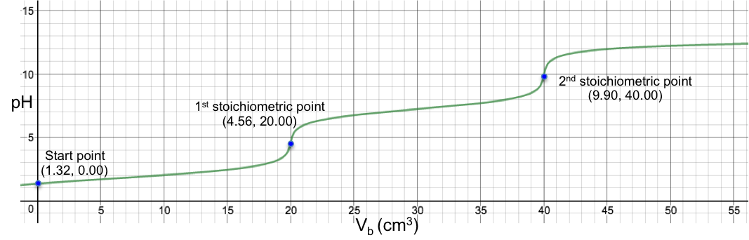
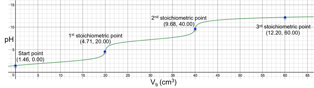
Eq19 is the complete pH titration curve for a diprotic acid (either strong or weak) versus monoprotic strong base system. We can input it in a mathematical software to generate a curve of pH against Vb. For example, if we titrate 10 cm3 of 0.200 M of H2SO4 (Ka1 = 1000, Ka2 = 1.02 x 10⁻²) with 0.100 M of NaOH, we have the following:
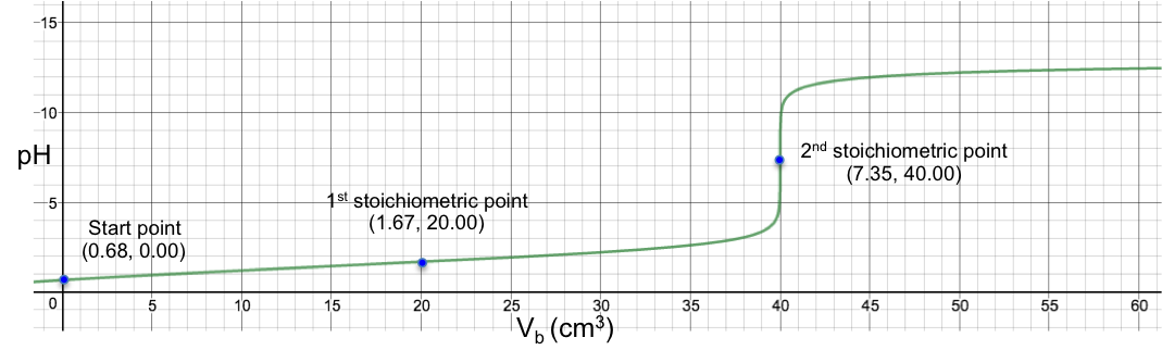
To understand the change in pH near the 1st stoichiometric point versus the change in Vb, we assume that one drop of base is about 0.05 cm3 and substitute 19.95 cm3, 20.00 cm3 and 20.05 cm3 into eq19. The respective pH just before and just after the 1st stoichiometric point (SP) are:
|
|
One drop before SP |
SP |
One drop after SP
|
|
Volume, cm3
|
19.95 |
20.00 |
20.05
|
|
pH
|
1.665 |
1.668 |
1.670
|
The data shows that two drops of base cause a change of only 0.005 in pH before and after the 1st stoichiometric point, which means we cannot monitor it during the titration process. The 1st stoichiometric point is not discernable as the 1st dissociation constant is a very large value, i.e. the first ionisation is complete. As for the 2nd stoichiometric point,
|
|
One drop before SP |
SP |
One drop after SP
|
|
Volume, cm3
|
39.95 |
40.00 |
40.05
|
|
pH
|
4.69 |
7.35 |
10.00
|
The data shows that just two drops of titrant cause a relatively big change of 5.31 in pH before and after the 2nd stoichiometric point. We can therefore use many different indicators that work within the range of the change in pH at the 2nd stoichiometric point to monitor the titration.
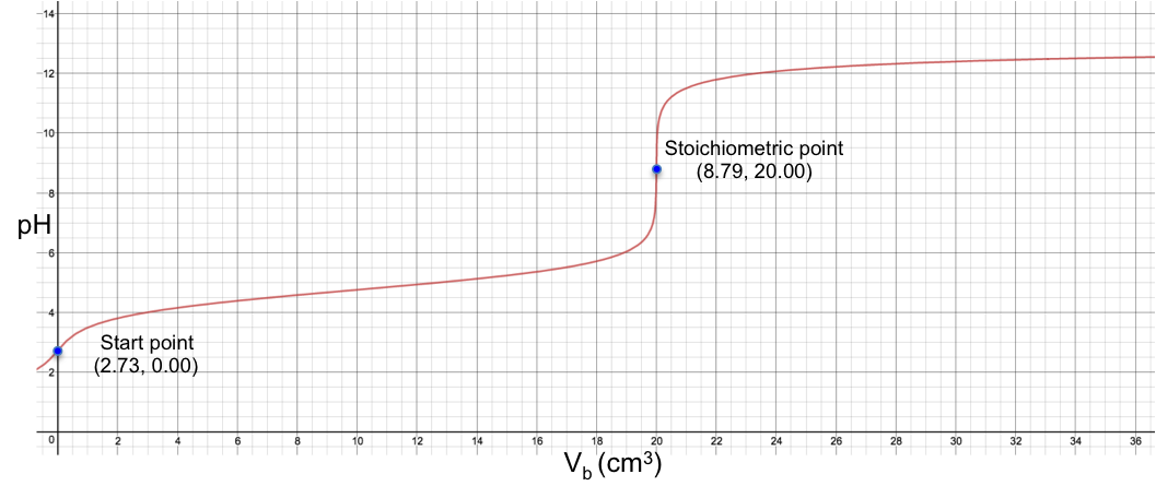
Another example is the titration of 10 cm3 of 0.200 M of H2CO3 (Ka1 = 4.5 x 10⁻⁷, Ka2 = 4.8 x 10⁻¹¹) with 0.100M of NaOH. Using eq19, we have:
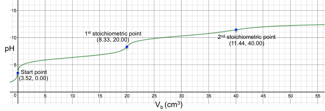
The changes of pH at both stoichiometric points are not sharp, with the 2nd one almost non-discernable. Finally, for the titration of 10 cm3 of 0.200 M of H2SO3 (Ka1 = 1.5 x 10⁻², Ka2 = 6.2 x 10⁻⁸) with 0.100M of NaOH, we have: