Intermediate Chemistry - Mono Mole

November 4, 2019November 30, 2024

Reaction mechanism (chemical kinetics)

A reaction mechanism is a stepwise molecular depiction of the way reactants interact to formed products in a chemical reaction. It is represented by one or more balanced chemical equations depending on whether the type of reaction it is describing is an elementary reaction or a complex reaction, respectively.

An elementary reaction is a chemical reaction where one or more species react in a single step to form products via a transition state. An example is the thermal decomposition of phosphorous (V) chloride:

$PCl_5\rightleftharpoons PCl_3+Cl_2$

Elementary reactions are classified according to their molecularity, which is the number of molecules reacting to form products in an elementary reaction.

Molecularity	Mechanism	Rate law	Order	Example
Unimolecular	$A\rightarrow P$	$rate=k[A]$	1^st	$PCl_5\rightleftharpoons PCl_3+Cl_2$
Bimolecular	$A+A\rightarrow P$	$rate=k[A]^2$	2^nd	$Br+Br\rightarrow Br_2$
Bimolecular	$A+B\rightarrow P$	$rate=k[A][B]$	2^nd	$CH_3Br+OH^-\rightleftharpoons CH_3OH+Br^-$
Trimolecular or Termolecular	$A+A+A\rightarrow P$	$rate=k[A]^3$	3^rd	$Cl+Cl+Cl\rightarrow Cl_2+Cl$
	$A+A+B\rightarrow P$	$rate=k[A]^2[B]$		$NO+NO+O_2\rightarrow 2NO_2$
	$A+B+C\rightarrow P$	$rate=k[A][B][C]$		$H+O_2+M\rightarrow HO_2+M$

A unimolecular reaction involves a species rearranging its bonds or dissociating to form products. Bimolecular and termolecular reactions occur when two and three molecules respectively collide to form products. The probability of elementary reactions involving the simultaneous collision of more than three molecules is very low.

From the table above, the rate law and hence the order of an elementary reaction can be predicted from the molecularity of the reaction, where unimolecular, bimolecular and termolecular reactions are, overall, first, second and third order reactions respectively.

As mentioned above, one or more species in an elementary reaction react via a transition state to form the products. The transition state is a point of highest potential energy on the potential energy profile curve of a reaction. It is where an unstable, transient and non-isolable chemical structure called an activated complex is formed (see diagram below).

For example, the bimolecular reaction between bromomethane and hydroxide ion to give methanol proceeds through the activated complex (denoted by $[\; \; ]^{\ddagger}$ ), where the C-Br bond weakens and the C-OH bond starts to form (see diagram below).

Complex reactions, on the other hand, occur through a series of steps. An example is the acid-catalysed iodination of propanone:

$CH_3COCH_3+I_2\; \; \begin{matrix} H^+\\\rightarrow \end{matrix}\; \; CH_3COCH_2I+HI$

The rate of the reaction depends on the concentration of two species but, surprisingly, does not depend on the concentration of iodine:

$rate=k[CH_3COCH_3][H^+]\; \; \; \; \; \; \; \; 42$

The mechanism of the reaction consists of four steps, each with a particular reaction rate (see diagram below).

The overall rate of reaction is dependent on the slowest step, which is called the rate determining step. As the rate determining step for the above reaction is the rearrangement of the first intermediate CH₃C(OH)CH₃⁺ to the second intermediate CH₃C(OH)CH₂, the proposed rate law is:

$rate=k_2\left [ CH_3C(OH)CH_3^+ \right ]\; \; \; \; \; \; \; \; 43$

However, in chemical kinetics, we are interested in analysing the effect of varying concentrations of reactants on the rate of the reaction. Therefore, we modify eq43 to reflect the concentrations of reactants by noting that

- k₂ « k_-1, such that we assume [CH₃C(OH)CH₃⁺] attains a constant value before the conversion of CH₃C(OH)CH₃⁺ to CH₃C(OH)CH₂ commences.
- The forward and reverse rates for the first step are equal at equilibrium and hence:

$k_1[CH_3COCH_3][H^+]=k_{-1}[CH_3C(OH)CH_3^{\; \: +}]$

$[CH_3C(OH)CH_3^{\; \: +}]=\frac{k_1}{k_{-1}}[CH_3COCH_3][H^+]\; \; \; \; \; \; \; \; 44$

Substitute eq44 in eq43

$rate=k[CH_3COCH_3][H^+]\; \; \; \; \; where\; \; k=\frac{k_1k_2}{k_{-1}}$

which is eq42.

An energy profile diagram of this reaction (see diagram above) shows four activated complexes with energies coinciding with the peaks (denoted by green dots) and three intermediates with potential energies matching the three troughs of the curve (denoted by red dots). It is important to note that an intermediate is a relative stable and isolable chemical species that exists for a finite time, while an activated complex is an unstable, non-isolable chemical structure that has only a transient existence.

Question

Propose a two-step mechanism for the reaction $2NO+O_2\rightarrow 2NO_2$ , which has the experimentally observed rate law: $rate=k[NO]^2[O_2]$ .

Answer

The rate determining step must involve O₂ or NO or both. Let’s suppose it is the final step of the mechanism and has O₂ as a reactant:

$M+O_2\; \; \begin{matrix} k_2\\\rightarrow \end{matrix}\; \; 2NO_2$

where M is an unknown intermediate molecule.

This implies that the preceding step is possibly:

$2NO\; \begin{matrix} k_1\\\rightleftharpoons \\ k_{-1} \end{matrix}\; M$

Balancing the above equations reveals the intermediate as: N₂O₂ . To check whether the proposed mechanism is reasonable, we write the rate law for the rate determining step:

$rate=k_2[N_2O_2][O_2]\; \; \; \; \; \; \; \; 45$

If we assume k₂ « k_-1 such that [N₂O₂] attains a constant value before it reacts with O₂, we can substitute the equilibrium expression of $k_1[NO][NO]=k_{-1}[N_2O_2]$ in eq45 to give:

$rate=k[NO]^2[O_2]\; \; \; \; \; where\; k=\frac{k_1k_2}{k_{-1}}$

To further validate the proposed mechanism, we need to isolate the intermediate.

Next article: Iodine clock

Previous article: Arrhenius equation

Content page of intermediate chemical kinetics

Content page of intermediate chemistry

Main content page

November 4, 2019November 20, 2025

Iodine clock experiment (chemical kinetics)

A typical iodine clock experiment seeks to determine the rate law of a reaction.

For the peroxide-iodide reaction $H_2O_2+2H^++2I^-\rightarrow 2H_2O+I_2$ , a proposed rate law is:

$rate=k[H_2O_2]^x[H^+]^y[I^-]^z\; \; \; \; \; \; \; \; 48$

Since the rate of the peroxide-iodide reaction is relatively slow, the method of initial rates can be used to determine the rate law. Let’s suppose a series of peroxide-iodide experiments is conducted at room temperature with the following parameters:

Experiment	Flask 1			Flask 2
Experiment	0.040M H₂O₂/cm³	0.05M H₂SO₄/cm³	Starch/ drops	0.010M KI /cm³	0.001M Na₂S₂O₃/cm³	H₂O/cm³
1	10	10	3	10	10	10
2	10	10	3	20	10	–
3	20	10	3	10	10	–
4	10	20	3	10	10	–

Water is added to experiment 1 so that all four experiments are conducted under the same constant volume. For every experiment, a stopwatch is turned on once the contents of the two flasks are mixed together and turned off when the mixture turns blue-black.

$H_2O_2+2H^++2I^-\rightarrow 2H_2O+I_2\; \; \; \; \; \; \; \; 49$

$2S_2O_3^{\; \: 2-}+I_2\rightarrow S_4O_6^{\; \: 2-}+2I^-\; \; \; \; \; \; \; \; 50$

When the mixture turns blue-black, the initial amount of 1.0×10^-5 moles of thiosulphate in each experiment has reacted with 5.0×10^-6 moles of iodine (eq50), which in turn required 1.0×10^-5 moles of iodide to produce (eq49). This means that we are measuring the time for a constant amount of 5.0×10^-6 moles of iodine to form in each experiment. Hence, we can rewrite eq48 as:

$\frac{d[I_2]}{dt}=\frac{\frac{n_{I_{2,f}}}{V}-\frac{n_{I_2,i}}{V}}{t_f-t_i}=k[H_2O_2]^x[H^+]^y[I^-]^z$

Since $n_{I_2,f}=5.0\times10^{-6}\: moles$ , $n_{I_2,i}=0$ , $V\approx0.05\, dm^3$ , and $t_i=0$

$\frac{\frac{5.0\times10^{-6}}{0.05}}{t_f}=k[H_2O_2]^x[H^+]^y[I^-]^z\; \; \; \; \; \; \; \; 51$

Comparing eq51 and eq48, $rate\propto\frac{1}{t_f}$ . Let’s assume that the experiment is completed with the different times $t_f$ recorded in the table below:

Experiment	Flask 1			Flask 2			Time (t_f)/s	(1/t_f)/10^-2 s^-1
Experiment	0.040M H₂O₂/cm³	0.05M H₂SO₄/cm³	Starch/ drops	0.010M KI /cm³	0.001M Na₂S₂O₃/cm³	H₂O/cm³	Time (t_f)/s	(1/t_f)/10^-2 s^-1
1	10	10	3	10	10	10	21.5	4.65
2	10	10	3	20	10	–	11.2	8.93
3	20	10	3	10	10	–	10.4	9.62
4	10	20	3	10	10	–	22.3	9.18

Comparing experiments 1 and 2, doubling the concentration of KI increases the reaction’s initial rate by $\frac{8.93}{4.65}=1.92$ or approximately two fold. From experiments 1 and 3, doubling the concentration of H₂O₂ increases the reaction’s initial rate by $\frac{9.62}{4.65}=2.07$ or approximately two fold. With reference to experiments 1 and 4, doubling the concentration of the acid increases the initial rate of the reaction by $\frac{9.17}{4.65}=1.97$ or approximately two fold. Notice that the factor, $\frac{5.0\times10^{-6}}{0.05}$ , disappears when we divide $\frac{\frac{5.0\times10^{-6}}{0.05}}{t_f}$ from different experiments to compare the initial reaction rates. Therefore, we use $\frac{1}{t_f}$ instead of $\frac{\frac{5.0\times10^{-6}}{0.05}}{t_f}$ to represent the initial reaction rates and conclude that the rate law is first order with respect to each reactant:

$rate=k[H_2O_2][H^+][I^-]$

NExt article: Radioactive decay

Previous article: Iodine clock

Content page of intermediate chemical kinetics

Content page of intermediate chemistry

Main content page

October 30, 2019October 11, 2025

Real gases: overview

Real gases deviate from ideal behaviour under high pressure and low temperature, exhibiting complex interactions and properties that are essential for understanding their characteristics in various scientific and industrial applications.

The ideal gas law functions well under conditions when gas particles are regarded as:

1. in constant random motion.
2. point masses with zero volume.
3. very far apart from one another
4. devoid of intermolecular forces of attraction or repulsion.
5. perfectly elastic.

Real gases, however, contain molecules that occupy a certain volume that is not negligible compared to the volume of the reaction vessel. Furthermore, intermolecular forces of attraction and repulsion between real gas molecules can be significant under certain conditions. Therefore, real gases deviate from ideality and require other equations of state to describe.

Next article: Compression factor

Content page of real gases

Content page of intermediate chemistry

Main content page

October 30, 2019January 23, 2025

Compression factor

The compression factor or compressibility factor measures the deviation of the behaviour a real gas from an ideal gas.

Intermolecular forces can be attractive or repulsive. Attractive forces have a longer range (several molecules in length) than repulsive forces.

Question

Why do attractive intermolecular forces have a longer range than repulsive intermolecular forces?

Answer

The difference in range between attractive and repulsive intermolecular forces boils down to the nature of these forces and how they act over distance. Attractive forces like van der Waals forces, dipole-dipole interactions, and hydrogen bonds decrease in strength more gradually with distance. For example, van der Waals forces decrease with the inverse sixth power of the distance between molecules. This means that even when molecules are relatively far apart, these forces can still exert a noticeable influence. Repulsive forces, on the other hand, are much stronger and decrease more rapidly with distance. These forces arise primarily from the overlap of electron clouds, leading to a strong repulsion due to the Pauli exclusion principle. The repulsive force increases exponentially as the distance between molecules decreases, making it significant only at very short distances.

At high pressures (high compression), repulsive forces between gas molecules are more significant than attractive forces, as the molecules occupy a small volume with small separations between them. The volume occupied by the gas is therefore expected to be larger than that for an ideal gas.

At low pressures (low compression), neither force is significant, as the gas molecules occupy a large volume with large separations between them. The gas therefore behaves ideally (i.e. volume occupied by the gas is expected to be the same as that for an ideal gas) and can be described mathematically by the ideal gas law.

At moderate pressures, attractive forces are more significant than repulsive forces, as the molecules are close enough for intermolecular attraction but not close enough for repulsive forces to be effective. The volume occupied by the gas is expected to be smaller than that for an ideal gas.

We can therefore measure the deviation of a real gas from ideality by analysing the ratio:

$Z=\frac{V_m}{V_m^{\: o}}\; \; \; \; \; \; \; \; 1$

where V_mis the molar volume of a gas, and V_m^o is the molar volume of an ideal gas at the same temperature and pressure as the gas of V_m.

We call this ratio, Z, the compression factor (or compressibility factor). The possible values of Z are as follows:

Pressure	Z
Low	1
Moderate	< 1
High	> 1

The diagram below shows the values of Z at different pressures for a few gases at the same temperature.

All gases have Z > 1 at high pressures (over 500 atm), Z < 1 at intermediate pressures (0 atm to 500 atm) and Z = 1 as p → 0. Since $V_m^{\: o}=\frac{RT}{p}$ , eq1 becomes

$pV_m=RTZ\; \; \; \; \; \; \; \; 2$

Eq2 is a simple equation of state that accounts for real gases when Z deviates from 1.

Question

Why is Z > 1 for H₂at intermediate pressures?

Answer

From eq2, Z is a function of temperature T. The diagram above shows a plot of Z for T > 100 K, where Z > 1 for H₂ at intermediate pressures. For T < 100 K, Z < 1 for H₂ at intermediate pressures. To elaborate further, H₂is smaller than the other gas molecules represented in the diagram. Therefore, we would expect repulsive forces between H₂molecules to be significant at higher pressures. In other words, H₂behaves like an ideal gas, with Z ≥ 1, at low and intermediate pressures for T > 100 K.

Next article: Critical constants

Previous article: Overview

Content page of real gases

Content page of intermediate chemistry

Main content page

October 30, 2019September 25, 2024

Critical constants

The critical constants of a real gas describe the conditions for liquefaction of the gas.

Thomas Andrews, an Irish chemist, conducted experiments on the liquefaction of gases in the 1860s and developed the concept of critical constants, which is summarised as follows:-

Consider a gas, Y, confined by a piston in a cylinder. The diagram below shows the pressure of the gas in the cylinder as the piston is pushed to vary the volume at various temperatures with T₁> T₂ > T₃ > T₄ > T₅. Each coloured line, called an isotherm, describes the change in pressure versus the change in molar volume of the gas at a specific temperature.

The isotherms at higher temperatures have smooth curves, while those at lower temperatures consist of horizontal portions. As we compress the gas at point A at temperature T₅, its pressure increases until just to the left of point B, where the gas starts to condense into its liquid form (it exists in both the liquid and gaseous phases with a defined surface separating the two). The system is now at equilibrium, where $Y(g)\rightleftharpoons Y(l)$ . The fact that the gas condenses into a liquid implies that it is a real gas (an ideal gas is devoid of intermolecular interactions).

As we manually compress the system further, more liquid is formed, as the system reacts according to Le Chatelier’s principle: the system counteracts the increase in pressure (decrease in volume) by shifting the position of the equilibrium of $Y(g)\rightleftharpoons Y(l)$ to the right to reduce the pressure, resulting in the pressure of the gas being constant. Hence, the curve from B to C is horizontal and is called a tie line. The pressure corresponding to the tie line is known as the vapour pressure of the liquid atT₅. At point C, all the gas is condensed into liquid with the piston touching the surface of the liquid.

The volume hardly changes when we compress the system further from C to D, as the liquid state of a substance is relatively incompressible. If we repeat the entire compression process at higher temperatures, we find that the width of the tie line shortens, e.g. for T₄, where it reduces to a maximum point (marked X) at T₃. We call this point the critical point of the substance and the isotherm that passes through it, the critical isotherm.

The temperature that produces the critical isotherm is called the critical temperature, T_c, e.g. T_cfor CO₂ is 31.04⁰C. The pressure and molar volume at the critical point is known as the critical pressure, p_c, and critical molar volume, V_c, respectively. p_c, V_c, and T_c are collectively called the critical constants of a substance.

The gas that is described by isotherms at temperatures above T_ccannot be compressed into a liquid regardless of the pressure applied. Due to the high pressure environment at temperatures above T_c, the gas has a density that is closer to that of a liquid and is called a supercritical fluid even though it is by definition a gas.

The density of a supercritical fluid and hence its solubility can be optimised for a particular application by adjusting its pressure. Supercritical CO₂, for example, is used to dissolve and extract caffeine from coffee beans and as a dry-cleaning solvent.

Generally, the regions shaded yellow, blue, pink and grey in the above graph represent the gas phase, the liquid-gas phase, the liquid phase and the supercritical fluid phase respectively.

Lastly, it is important to note that at points B, C, X and all other points on the boundary separating the liquid-gas zone from the other zones, the substance exists only in one phase. For example, at the critical point, the meniscus between the liquid and gas (supercritical fluid) phases disappears, as there is no difference in densities of the liquid and gas (supercritical fluid).

Next article: van der Waal’s equation of state

Previous article: Compression factor

Content page of real gases

Content page of intermediate chemistry

Main content page

October 30, 2019December 5, 2024

van der Waal’s equation of state

Johannes van der Waals, a Dutch physicist, introduced an equation in 1873 called the van der Waals equation to mathematically describe the physical state of a real gas.

This equation is:

$\left [ p+a\left ( \frac{n}{V} \right )^2 \right ]\left ( V-nb \right )=nRT\; \; \; \; \; \; \; \; 3$

where a and b are called the van der Waals coefficients, which are temperature-independent constants specific to each gas.

The equation looks similar to the ideal gas equation except for the pressure and volume factors of $a\left ( \frac{n}{V} \right )^2$ and nb, respectively. To understand how van der Waals’ equation is derived, we need to know how the ideal gas law is conceptualised.

The ideal gas equation, pV = nRT, is derived from the combined experiments of Robert Boyle and Jacques Charles, and a principle developed by Amedeo Avogadro. This means that, for a fixed amount of gas at a relatively high temperature, the product of the experimentally observed values of p and V in the equation is a constant. The equation works reasonably well at low pressures where gases approach ideality. Under such conditions, gas particles can be assumed to be point masses with zero volume and, therefore, have no intermolecular forces of attraction or repulsion between them. In other words, the equation only works when the observed variables of p and V are ‘ideal’:

$p_{ideal}V_{ideal}=nRT\; \; \; \; \; \; \; \; 4$

In reality, gases have finite volumes and repel one another, especially at high pressures. The experimentally observed values of pressures and volumes are actually p_real and V_real. Therefore, for eq4 to work, we have to modify it.

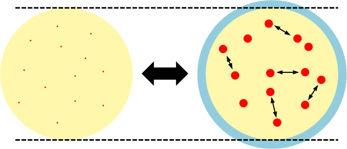
Due to the presence of repulsive forces between real gas molecules at high pressures, the observed volume of a real gas is larger than the volume of its ideal counterpart, that is, V_real > V_ideal. The diagram below shows the volume expansion (from yellow to blue) if the point masses have finite volumes.

Letting the difference in molar volume of a real gas and an ideal gas be b, we have $\frac{V_{real}}{n}-\frac{V_{ideal}}{n}=b$ or

$V_{ideal}=V_{real}-nb\; \; \; \; \; \; \; \; 5$

Substituting eq5 in eq4 and rearranging yields

$V_{real}=\frac{nRT}{p_{ideal}}+nb\; \; \; \; \; \; \; \; 6$

Eq6 predicts that the molar volume of a gas at zero Kelvin is b. Experiments indeed reveal that b has approximately the same value as the molar volume of the solid form or liquid form of the gas near that temperature. On the other hand, the ideal gas law, $V_{ideal}=\frac{nRT}{p_{ideal}}$ , wrongly predicts that the volume of a gas at 0 K is zero.

Next, the pressure that a real gas exerts on the wall of a container is lower than the pressure of its ideal counterpart (p_ideal > p_real), as the molecules of a real gas experience intermolecular forces of attraction that decelerates their motion when they are about to impact the wall of the container. This means that we need to add a pressure shortfall, Δp_real, to the observed real pressure to reflect the ideal pressure that fits eq4:

$p_{ideal}=p_{real}+\Delta p_{real}\; \; \; \; \; \; \; \; 7$

If we perceive the intermolecular force of attraction (i.e., the force that one molecule of gas experiences near the wall of the container) as the attraction between that molecule and the bulk of the gas, the pressure shortfall due to that particular molecule is proportional to the density of the gas:

$\Delta p_{real,\, one\, molecule}=k\left ( \frac{n}{V_{real}} \right )$

Furthermore, the total number of molecules N near the wall of the container is again proportional to the density of the gas:

$N=k'\left ( \frac{n}{V_{real}} \right )$

The total pressure shortfall is therefore:

$\Delta p_{real}=N\Delta p_{real,\, one\, molecule}=k'\left ( \frac{n}{V_{real}} \right )k\left ( \frac{n}{V_{real}} \right )=a\left ( \frac{n}{V_{real}} \right )^2$

where a = k’k is a proportionality constant specific to a particular gas.

Eq7 becomes

$p_{ideal}=p_{real}+a\left ( \frac{n}{V_{real}} \right )^2\; \; \; \; \; \; \; \; 8$

Substituting eq5 and eq8 in eq4, we get the explicit form of eq3:

$\left [ p_{real}+a\left ( \frac{n}{V_{real}} \right )^2 \right ]\left ( V_{real}-nb \right )=nRT\; \; \; \; \; \; \; \; 9$

The pressure and volumes in eq9 now represent experimentally observed real pressure and real volumes, respectively. We have essentially converted an equation that only works for ideal gases into one that is applicable for real gases. For simplicity, we can omit the subscripts, which gives eq3.

Using eq3, the van der Waals equation can also be expressed in the molar form by substituting it with the molar volume, $V_m=\frac{V}{n}$ , to give:

$\left ( p+\frac{a}{V_m^{\: 2}} \right )\left ( V_m-b \right )=RT$

which rearranges to:

$p=\frac{RT}{V_m-b}-\frac{a}{V_m^{\: 2}}\; \; \; \; \; \; \; \; 10$

At high molar volumes (i.e. low pressures), V_m – b ≈ V_m and the second term on the RHS of eq10 becomes very small, with eq10 reducing to the ideal gas equation: $p\approx \frac{RT}{V_m}$ .

The van der Waals equation is an improvement over eq2, as it is able to describe the physical state of a real gas in terms of the van der Waals coefficients a and b, which relate to the strength of the forces of attraction between molecules and the size of the molecules, respectively.

Since the critical isotherm of a gas has an inflexion point at the critical point, we can determine the van der Waals coefficients for a gas by finding the 1^st and 2^nd derivatives of eq10, letting these be equal to zero and solving for the critical constants:

$\frac{dp}{dV_m}=-\frac{RT}{\left ( V_m-b \right )^2}+\frac{2a}{V_m^{\: 3}}=0\; \; \; \; \; \; \; \; 11$

$\frac{dp}{dV_m}=\frac{2RT}{\left ( V_m-b \right )^3}-\frac{6a}{V_m^{\:4}}=0\; \; \; \; \; \; \; \; 12$

From eq11 and eq12, $a=\frac{RTV_c^{\: 3}}{2\left ( V_c-b \right )^2}$ and $a=\frac{RTV_c^{\: 4}}{3\left ( V_c-b \right )^3}$ respectively. Combining both values of a,

$V_c=3b\; \; \; \; \; \; \; \; 13$

Substitute eq13 back in eq11 where V_m is now V_c,

$T_c=\frac{8a}{27Rb}\; \; \; \; \; \; \; \; 14$

Substitute eq13 and eq14 back in eq10,

$p_c=\frac{a}{27b^2}\; \; \; \; \; \; \; \; 15$

Hence, by measuring the pressure, volume and temperature at the critical point of a gas (i.e. the critical constants), we can calculate the van der Waals coefficients for that gas. The table below shows the van der Waals coefficients for some common gases:

	a / atm dm⁶mol^-2	b / 10^-2 dm³mol^-1
H₂	0.2420	2.65
N₂	1.352	3.87
O₂	1.364	3.19
CO₂	3.610	4.29

Next article: Virial equation of state

Previous article: Critical constants

Content page of real gases

Content page of intermediate chemistry

Main content page

October 30, 2019September 25, 2024

Virial equation of state

The virial equation of state is a mathematical expression that models the behaviour of a real gas.

Recognising van der Waals’ work, Heike Kamerlingh, another Dutch physicist, attempted to establish a more extensive equation of state and devised the virial equation of state in 1882:

$pV_m=RT\left ( 1+\frac{B}{V_m}+\frac{C}{V_m^{\: 2}}+... \right )\; \; \; \; \; \; \; \; 16$

The word virial is latin meaning force or energy. The RHS of eq16 suggests that the virial equation is derived using a power series.

In fact, the equation can be perceived as a Maclaurin series of van der Waals’ equation. To illustrate this, let’s multiply the right side of eq10 from the previous section by $\frac{x}{x}$ where $x=\frac{1}{V_m}$ to give:

$p=\frac{RTx}{1-bx}-ax^2\; \; \; \; \; \; \; \; 17$

A Maclaurin series for the polynomial $p(x)=c_0+c_1x+c_2x^2+c_3x^3+...$ is in the form:

$p(x)=p(0)+\frac{p'(0)}{1!}x+\frac{p''(0)}{2!}x+\frac{p'''(0)}{3!}x+...\; \; \; \; \; \; \; \; 18$

From eq17,

$p(0)=0\; \; \; \; \; \; 19$

$p'(0)=\frac{RT(1-bx)+bRTx}{(1-bx)^2}-2ax=RT\; \; \; \; \; \; \; 20$

$p''(0)=\frac{2b\left [ RT(1-bx)+bRTx \right ](1-bx)}{(1-bx)^4}-2a=2(bRT-a)\; \; \; \; \; \; \; 21$

$p'''(0)=\frac{6b^2RT}{(1-bx)^4}=6b^2RT\; \; \; \; \; \; \; 22$

Substituting eq19 through eq22 in eq18

$p(x)=RTx\left [ 1+\left ( b-\frac{a}{RT} \right )x+b^2x^2+... \right ]\; \; \; \; \; \; \; \; 23$

Substitute $x=\frac{1}{V_m}$ back in eq23

$p(x)=\frac{RT}{V_m}\left [ 1+\frac{\left ( b-\frac{a}{RT} \right )}{V_m}+\frac{b^2}{V_m^{\: 2}}+... \right ]\; \; \; \; \; \; \; \; 24$

Eq24 is the same as eq16 if $B=\left ( b-\frac{a}{RT} \right )$ and C = b². If so, the coefficient C (and perhaps other higher coefficients) is not a function of temperature, which limits the accuracy of the equation in predicting the pressure of the real gas. Kamerlingh therefore decided to use experimental data to determine the coefficients B, C and so on, instead of using the van der Waals factors, resulting in eq16 as the final form rather than eq24.

Comparing eq16 and eq2, the compression factor is equal to the expansion part of the virial equation

$Z=1+\frac{B}{V_m}+\frac{C}{V_m^{\: 2}}+...$

If all the virial coefficients are equal to zero, Z = 1 and the virial equation becomes the ideal gas equation. For large V_m (i.e. at low pressures), all the terms with virial coefficients tend to zero with the virial equation transforming into the ideal gas equation again. The virial equation can also be expressed in terms of powers of pressure:

$pV_m=RT\left ( 1+B'p+C'p^2+... \right )\; \; \; \; \; \; \; \; 25$

The pressure version of the virial equation is constructed in a way that is consistent with the volume version, such that the equation becomes the ideal gas equation when all the virial coefficients are zero.

In summary, the virial equation’s accuracy in modeling the behaviour of real gases increases with increasing number of expansion terms. However, it may be cumbersome to determine the virial coefficients that are needed to make the equation work.

Previous article: van der Waal’s equation of state

Content page of real gases

Content page of intermediate chemistry

Main content page

October 26, 2019October 5, 2025

Chemical equilibrium: overview

Chemical equilibrium occurs when the rates of the forward and reverse reactions in a dynamic system become equal, resulting in constant concentrations of reactants and products despite ongoing processes.

Some chemical reactions are reversible (i.e. the products can react to re-form the reactants), e.g.

$PCl_5(g)\rightleftharpoons PCl_3(g)+Cl_2(g)$

Such reactions are denoted by the double harpoon sign $\rightleftharpoons$ , instead of the single arrow sign → for irreversible reactions.

Consider only the presence of PCl₅ in a closed, heated reaction vessel at the start of the reaction. Initially, PCl₅ molecules collide with each other to form PCl₃and Cl₂ at a relatively high rate, as both the temperature and the concentration of PCl₅ are high. As some PCl₃and Cl₂ are formed, they also begin to collide and re-form PCl₅, but at a relatively slower rate. Over time, the decreasing concentration of PCl₅ and the increasing concentrations of PCl₃and Cl₂ reach a point where the forward reaction rate equals the reverse reaction rate, resulting in no net change in the concentrations of the reactant PCl₅ and the products PCl₃and Cl₂. We say that the reaction has attained dynamic equilibrium when it reaches such a state. The course of the reaction is represented by the graph below:

It is important to note that a closed system is necessary for a reaction to achieve chemical equilibrium.

Next article: Equilibrium constant

Content page of chemical equilibrium

Content page of intermediate chemistry

Main content page

October 26, 2019September 22, 2025

Units of the equilibrium constant

The thermodynamic definition of the equilibrium constant K (see this advanced level article for derivation) is

$\Delta_rG^{\: o}=-RTlnK$

where Δ_rG^o is the reaction Gibbs energy at standard conditions (a constant for a particular reaction), R is the gas constant, T is temperature.

Since logarithms only take pure numbers, K is a dimensionless number. However, when equilibrium constants are calculated as a quotient of concentrations or partial pressures, the practice is to quote them in units of concentration or pressure according to the quotient.

$K_c=\frac{\left [ C \right ]^p\left [ D \right ]^q...}{\left [ A \right ]^m\left [B \right ]^n...}\; \; \; or\; \; \; K_p=\frac{p_C^{ \; \; \; p}p_D^{ \; \; \;q}...}{p_A^{ \; \; \; m}p_B^{\; \; \; n}...}$

For example, the units of K_c for

$K_c=\frac{\left [ CoCl_4^{\; 2-} \right ]}{\left [ Co\left ( H_2O \right )_6^{\; 2+} \right ]\left [ Cl^- \right ]^4}$

is mol^-4dm¹².

Next article: The relationship between K_p and K_c

Previous article: Equilibrium constant

Content page of chemical equilibrium

Content page of intermediate chemistry

Main content page

October 26, 2019September 25, 2024

Equilibrium constant

The equilibrium constant of a chemical reaction describes the relationship between the concentrations of the reactants and the concentrations of the products of the reaction at dynamic equilibrium.

Chemists found that when a reversible reaction reaches dynamic equilibrium, the product of the concentrations (or partial pressures) of the reaction products raised to the power of their stoichiometric coefficients divided by the product of the concentrations (or partial pressures) of the reactants raised to the power of their stoichiometric coefficients, has a constant value at a particular temperature (see this advanced level article for derivation). For the decomposition of PCl₅ at 620K,

$PCl_5(g)\rightleftharpoons PCl_3(g)+Cl_2(g)$

we have

$K_c=\frac{\left [ PCl_3 \right ]\left [ Cl_2 \right ]}{\left [ PCl_5 \right ]}$

where [i] is the concentration in mol dm^-3 of the species i.

We called this constant, K_c, the equilibrium constant. Since the species in this reaction are in the gaseous state and that the partial pressure of gas is proportional to its concentration, we can also express the equilibrium constant of this reaction in terms of partial pressures of the species:

$K_p=\frac{P_{PCl_3}P_{Cl_2}}{P_{PCl_5}}$

where p_i is the partial pressure of gas i and K_p is the equilibrium constant in terms of partial pressures. Note that K_c may or may not be equal to K_p for a particular reaction (see here for details).

Another example is the reaction:

$N_2(g)+3H_2(g)\rightleftharpoons 2NH_3(g)$

where

$K_c=\frac{\left [ NH_3 \right ]^2}{\left [ N_2 \right ]\left [ H_2 \right ]^3}\; \; \; or\; \; \; K_p=\frac{P_{NH_3}^{\; \; \; \; \; \; 2}}{P_{N_2}P_{H_2}^{\; \; \; \; 3}}$

In general, for a reaction

$mA+nB+...\rightleftharpoons pC+qD+...$

Question

Calculate the equilibrium constant for the dissociation of PCl₅ in a 250 ml vessel if the initial and equilibrium amounts of the reactant are 0.0175 mol and 0.0125 mol respectively (assuming no products formed initially).

Answer

	PCl₅	PCl₃	Cl₂
Initial conc, M	0.0175/0.250	0	0
Equilibrium conc, M	0.0125/0.250	(0.0175-0.0125)/0.250	(0.0175-0.0125)/0.250

$K_c=\frac{\frac{0.0050}{0.250}\frac{0.0050}{0.250}}{\frac{0.0125}{0.250}}=8.0\times 10^{-3}\: M$

Question

Answer

Next article: Iodine clock

Previous article: Arrhenius equation

NExt article: Radioactive decay

Previous article: Iodine clock

Next article: Compression factor

Question

Answer

Question

Answer

Next article: Critical constants

Previous article: Overview

Next article: van der Waal’s equation of state

Previous article: Compression factor

Next article: Virial equation of state

Previous article: Critical constants

Previous article: van der Waal’s equation of state

Next article: Equilibrium constant

Next article: The relationship between Kp and Kc

Previous article: Equilibrium constant

Question

Answer

Next article: Units of Equilibrium constant

Previous article: Overview

Next article: The relationship between K_p and K_c