The rate of a reaction has been defined in a basic level article as:
For a simple reaction, A → B at constant volume V1, we can define its rate as
where nB is the amount of B.
Since the rate of formation of product must be the same as the rate of consumption of the reactant, and that the rate of a reaction is defined as a positive value, we have: .
Suppose we have another reaction, C → D at a different constant volume V2, with a rate:
To have a meaningful comparison of the rates of these two reactions with different reacting volumes, we need a common basis, which can be obtained by dividing eq2 and eq3 by their respective volumes. Therefore, a better definition of the rate of a reaction is:
Consider an experiment where HCl is added to CaCO3 to produce CO2 in a rigid vessel with a pressure gauge. The data collected are presented in a CO2 pressure versus time plot. If we use a constant mass of CaCO3 and 3 different concentrations of 20 cm3 of HCl, we have 3 different gradients at the origin, which represent 3 initial rates of reaction (see diagram below) with RA corresponding to the reaction with the highest concentration of HCl and RC relating to the reaction with the lowest concentration of HCl.
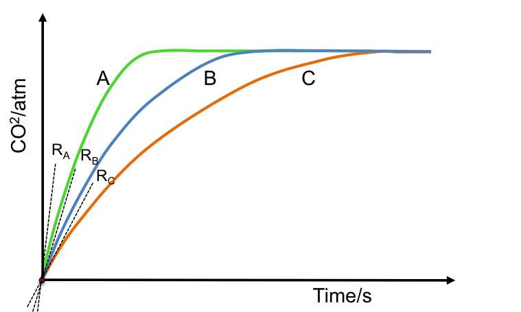
The above results imply that the rate of reaction is proportional to the concentration of the reactant used. Therefore, in addition to eq4, we can also expressed the rate of a reaction in the form of an equation known as a rate law:
where [H3O+] is the concentration of hydroxonium ions from HCl and k is a proportionality constant called the rate constant. Combining eq4 and eq5,
Eq6 means that an increase in concentration of hydroxonium ions increases the rate of change in concentration of CO2, which is measured by the rate of change in pressure of CO2, since .