Intermediate Chemistry - Mono Mole

November 4, 2019October 14, 2024

Isolation method (chemical kinetics)

Isolation methods are used for reactions with multiple reactants, e.g.

$A+B\rightarrow C+D$

$rate=k\left [ A \right ]^{i} \left [ B \right ]^{j}\; \; \; \; \; \; \; \; 35$

There are two isolation methods to determine the rate of a reaction. The first, which is used together with the initial rate method, involves varying the concentration of one of the reactants A, while keeping the concentration of the other reactant B constant. The initial rates of these reactions are then determined. Since the concentration of Bis constant for all the experiments and that initial rates are used, eq35 becomes

$initial\: rate=k\, '\left [ A \right ]_0^{\: i}\; \; \; \; \; \; \; \; 36$

where $k\, '=k\left [ B \right ]_0^{\: j}$

By isolating the reactant of interest, A, eq35 has changed from an (i + j) order equation to a pseudo-i order equation. Taking the natural logarithm of both sides of eq36 and plotting the experimental results in a ln(initial rate) versus ln[A]₀graph, we can find the gradient of the curve, which is the order with respect to A, and the vertical intercept of the curve, which corresponds to ln(k[B]₀ ^j). To find j and hence the value of k, we repeat the series of experiments by varying concentrations of B while keeping the concentration of A constant, and carrying out the same graphical analysis as before.

The second isolation method involves using an excess amount of one reactant, e.g. B, such that its concentration remains unchanged during the prolonged course of the reaction. Eq35 becomes

$rate=k''\left [ A \right ]^{i}\; \; \; \; \; \; \; \; 37$

$ln\left ( rate \right )=iln\left [ A \right ]+lnk''\; \; \; \; \; \; \; \; 38$

where $k''=k\left [ B \right ]^{j}$

With just a single experiment, the gradients at various points on the curve of a [A] versus time graph correspond to the reaction rates at different [A]. These data are then used to construct another graph with eq38 to determine i and lnk”. Similarly, to find k and j, we repeat the experiment, this time with [A] in excess and carry out the same graphical analysis as before.

Question

Can the first isolation method be used without the initial rate method, i.e. can we, with the first isolation method, let the reaction run its course as per the situation in eq37?

Answer

No. This is because the concentration of the reactant that is kept constant is not in excess. The concentration of that reactant will change during the course of the reaction, rendering k” a variable. In other words, the concentration of the reactant that is kept constant in the first method is only constant during the duration necessary for the initial rate of the reaction to be taken.

Next article: Arrhenius equation

Previous article: Why is Initial rate proportional to 1/t?

Content page of intermediate chemical kinetics

Content page of intermediate chemistry

Main content page

November 4, 2019December 12, 2024

Why is initial rate proportional to 1/t?

The ‘initial rate proportional to 1/t’ concept is applicable to a chemical kinetics experiment that has the initial concentration of a reactant varied but the measured amount of a product fixed. One such experiment is the decomposition of hydrogen peroxide over a platinum catalyst, while another is the iodine clock. For the decomposition experiment, we have:

$2H_2O_2(aq)\rightleftharpoons2H_2O(l)+O_2(g)$

Using various initial concentrations of H₂O₂, different times taken to collect a fixed volume of oxygen are recorded. The diagram below illustrates the setup, where the fixed volume of oxygen produced under constant temperature is measured by a fixed change in pressure of the constant-volume system.

Since the reaction is very slow, we assume that the initial concentration of H₂O₂ for each experiment remains relatively unchanged for the volume of oxygen generated (the change in pressure of the system can be fixed at an amount that does not exceed three minutes to occur). Using eq10, and assuming gases behave ideally, we can write

$initial\, rate=\frac{d[O_2]}{dt}=\frac{\Delta (n_{O_2}/V)}{\Delta t}=\frac{\Delta p}{RT\Delta t}\; \; \; \; \; \; \;\; 27$

To produce a fixed volume of oxygen, the change in amount of oxygen, and hence the change in pressure of the system, is constant regardless of the concentration of H₂O₂ used. Thus,

$initial\, rate=C\frac{1}{\Delta t}\; \; \; \; \; \; \; \; 28$

where C is a constant and is equal to $\frac{\Delta p}{RT}$ .

This answers the question of why initial rate is proportional to 1/t.

To develop an equation that that allows us to further analyse the decomposition reaction, we propose the following rate law:

$initial\, rate=k[H_2O_2]_0^{\;\: i}\; \; \; \; \; \; \; \; 29$

where [H₂O₂]₀is the initial concentration of H₂O₂.

Taking the natural logarithm for both sides of eq28 and eq29, we have

$ln(initial\, rate)=ln\frac{1}{\Delta t}+ln\frac{\Delta p}{RT}\; \; \; \; \; \; \; \; 30$

and

$ln(initial\, rate)=iln[H_2O_2]_0+lnk\; \; \; \; \; \; \; \; 31$

Substitute eq31 in eq30

$ln\frac{1}{\Delta t}=iln[H_2O_2]_0+ln\frac{k}{\Delta p/RT}\; \; \; \; \; \; \; \; 32$

Therefore, using the time measurements for the fixed change in pressure to occur for different initial concentrations of H₂O₂, a plot of $ln\frac{1}{\Delta t}$ versus $ln[H_2O_2]_0$ gives a gradient of the order of the reaction, i, and a vertical intercept of $ln\frac{k}{\Delta p/RT}$ where k is the rate constant.

Question

Eq32 is derived using the rate equation $\frac{d[O_2]}{dt}=k[H_2O_2]_0^{\; \, i}$ . What if we define the rate equation as $-\frac{1}{2}\frac{d[H_2O_2]}{dt}=k_1[H_2O_2]_0^{\; \, i}$ ?

Answer

$-\frac{1}{2}\frac{\Delta n_{H_2O_2}/V_{H_2O_2}}{\Delta t}=k_1[H_2O_2]_0^{\: \, i}$

$ln\left ( -\frac{1}{2}\frac{\Delta n_{H_2O_2}}{V_{H_2O_2}} \right )+ln\frac{1}{\Delta t}=lnk_1+iln[H_2O_2]_0$

$ln\frac{1}{\Delta t}=iln[H_2O_2]_0+ln\left ( \frac{k_1}{-\Delta n_{H_2O_2}/2V_{H_2O_2}} \right )\; \; \; \; \; \; \; \; 33$

To produce a fixed volume of oxygen, the change in amount of H₂O₂, $\Delta n_{H_2O_2}$ , is a constant value regardless of the initial amounts of H₂O₂. For example, to produce 1 mole of oxygen, the change in amount of H₂O₂ is always -2 moles irrespective of how many moles of H₂O₂ there are to begin with. Furthermore, the same volume of H₂O₂is used as we vary [H₂O₂]. So, the 2^nd term on RHS of eq33 is a constant, which makes eq33, like eq32, a linear function.

Comparing eq33 with eq32,

$k_1=-\frac{\Delta n_{H_2O_2}RT}{2V_{H_2O_2}\Delta p}k$

Next article: Isolation method

Previous article: Initial rate method

Content page of intermediate chemical kinetics

Content page of intermediate chemistry

Main content page

November 4, 2019September 25, 2024

Arrhenius equation (chemical kinetics)

The Arrhenius equation was conceived by Svante Arrhenius, a Swedish chemist, in 1889.

It relates the rate constant, k, of a reaction with the temperature of the reaction, T, as follows:

$k=Ae^{-\frac{E_a}{RT}}\; \; \; \; \; \; \; \; 39$

where E_a is the activation energy of the reaction, R is the universal gas constant and A is the pre-exponential factor. The values of E_a and A of a reaction are experimentally determined.

The Arrhenius equation is based on the van’t Hoff equation: $\Delta_rH^o=RT^2\frac{dlnK}{dT}$ . Consider a reversible elementary reaction $A+B\; \; \begin{matrix} k_1\\\rightleftharpoons \\ k_2 \end{matrix}\; \; P$ , where k₁and k₂ are the rate constants of the forward and reverse reactions respectively. At equilibrium, $rate_1=rate_2$ and therefore, $k_1[A][B]=k_2[P]$ or $\frac{k_1}{k_2}=\frac{[P]}{[A][B]}=K$ . Substituting $K=\frac{k_1}{k_2}$ in the van’t Hoff equation,

$\Delta_rH^o=RT^2\frac{dlnk_1}{dT}-RT^2\frac{dlnk_2}{dT}$

If we define $RT^2\frac{dlnk}{dT}=E_a$ ,

$\Delta_rH^o=E_{a1}-E_{a2}\; \; \; \; \; \; \; \; 40$

Eq40 is best interpreted using a potential energy graph:

The definition of activation energy, $E_a=RT^2\frac{dlnk}{dT}$ , results in eq39 when integrated. Taking the natural logarithm on both sides of eq39,

$lnk=lnA-\frac{E_a}{RT}\; \; \; \; \; \; \; \; 41$

Eq41 is a linear function with dependent variable $lnk$ and independent variable $\frac{1}{T}$ , so that a plot of $lnk$ versus $\frac{1}{T}$ gives a gradient of $-\frac{E_a}{R}$ and vertical intercept of $lnA$ .

Question

Are the activation energy E_a and pre-exponential factor A of a reaction independent of temperature?

Answer

For the Arrhenius equation to be applicable, a plot of lnk versus 1/T must, with strong linear correlation, produce a straight line when values of k at various T are substituted in eq41. This implies that the activation energy E_a and pre-exponential factor A of a reaction are constants and therefore independent of temperature. In fact, the Arrhenius equation works reasonably well for many reactions over a temperature range of about 100 K. However, deviations from the equation do occur for some other reactions.

A more rigorous approach to analyse the relation between k and T using the transition state theory (TST) reveals the temperature-dependence of the activation energy of a reaction, with $E_a=\Delta^{\ddagger}H^o+xRT$ , where x = 1 for unimolecular gas-phase reactions and x = 2 for bimolecular gas-phase reactions. The TST also shows that the pre-exponential factor is dependent on temperature, where $A=\frac{\kappa e^xkRT}{p^oh}^2e^{\frac{\Delta^{\ddagger}S^o}{R}}$ .

So why does the Arrhenius equation work for so many reactions when both the activation energy and pre-exponential factor of a reaction are temperature-dependent? For E_a, the value $\Delta^{\ddagger}H^o$ is usually much bigger than xRT, and for A, T²is dwarfed by the term $\frac{\kappa e^xkR}{p^oh}e^{\frac{\Delta^{\ddagger}S^o}{R}}$ .

Next article: REaction mechanism

Previous article: Isolation method

Content page of intermediate chemical kinetics

Content page of intermediate chemistry

Main content page

November 4, 2019September 25, 2024

Iodine clock (chemical kinetics)

The iodine clock is a chemical clock experiment devised by Hans Landolt, a Swiss chemist, in 1886. It illustrates the theories of chemical kinetics and redox chemistry via reactions that generate aqueous iodine as a product, and manifests the concept of a chemical clock through the time taken by one or more parallel reactions to consume the iodine produced.

An example is the oxidation of iodide by hydrogen peroxide to form aqueous iodine:

$H_2O_2+2H^++2I^-\rightarrow 2H_2O+I_2\; \; \; \; \; \; \; \; 46$

The iodine produced immediately reacts with a known amount of reducing agent, e.g. sodium thiosulphate, which is added to the peroxide-iodide mixture together with some starch solution at the start of the reaction.

$2S_2O_3^{\; \: 2-}+I_2\rightarrow S_4O_6^{\; \: 2-}+2I^-\; \; \; \; \; \; \; \; 47$

As the thiosulphate-iodine reaction occurs at a much faster rate than the peroxide-iodide reaction and it regenerates the exact stoichiometric amount of iodide ions that is present at the start of the reaction, the presence of iodine is only detected when all of the thiosulphate has been reacted.

When there is no more thiosulphate to remove the iodine, iodine combines with the unreacted iodide to form the triiodide ion, which in turn forms an intense blue-black charge-transfer complex with starch:

$I_2+I^-\rightleftharpoons I_3^{\; \; -}\; \; \begin{matrix} starch\\\rightarrow \end{matrix}\; \; coloured\, complex$

The different times needed for the mixtures to turn blue-black are recorded for a series of experiments using different concentrations of hydrogen peroxide, acid and iodide. For a constant amount of thiosulphate, the longer the time taken for the mixture to turn blue-black, the slower the peroxide-iodide reaction. In other words, the rate of the peroxide-iodide reaction is inversely proportional to the time taken for the mixture to turn blue-black.

Another version of the iodine clock experiment is the reaction between ammonium persulphate and potassium iodide:

$S_2O_8^{\; \; 2-}+2I^-\rightarrow 2SO_4^{\; \; 2-}+I_2$

$I_2+2S_2O_3^{\; \; 2-}\rightarrow2I^-+S_4O_6^{\; \; 2-}$

Next article: Iodine clock experiment

Previous article: Reaction mechanism

Content page of intermediate chemical kinetics

Content page of intermediate chemistry

Main content page

November 4, 2019November 30, 2024

Reaction mechanism (chemical kinetics)

A reaction mechanism is a stepwise molecular depiction of the way reactants interact to formed products in a chemical reaction. It is represented by one or more balanced chemical equations depending on whether the type of reaction it is describing is an elementary reaction or a complex reaction, respectively.

An elementary reaction is a chemical reaction where one or more species react in a single step to form products via a transition state. An example is the thermal decomposition of phosphorous (V) chloride:

$PCl_5\rightleftharpoons PCl_3+Cl_2$

Elementary reactions are classified according to their molecularity, which is the number of molecules reacting to form products in an elementary reaction.

Molecularity	Mechanism	Rate law	Order	Example
Unimolecular	$A\rightarrow P$	$rate=k[A]$	1^st	$PCl_5\rightleftharpoons PCl_3+Cl_2$
Bimolecular	$A+A\rightarrow P$	$rate=k[A]^2$	2^nd	$Br+Br\rightarrow Br_2$
Bimolecular	$A+B\rightarrow P$	$rate=k[A][B]$	2^nd	$CH_3Br+OH^-\rightleftharpoons CH_3OH+Br^-$
Trimolecular or Termolecular	$A+A+A\rightarrow P$	$rate=k[A]^3$	3^rd	$Cl+Cl+Cl\rightarrow Cl_2+Cl$
	$A+A+B\rightarrow P$	$rate=k[A]^2[B]$		$NO+NO+O_2\rightarrow 2NO_2$
	$A+B+C\rightarrow P$	$rate=k[A][B][C]$		$H+O_2+M\rightarrow HO_2+M$

A unimolecular reaction involves a species rearranging its bonds or dissociating to form products. Bimolecular and termolecular reactions occur when two and three molecules respectively collide to form products. The probability of elementary reactions involving the simultaneous collision of more than three molecules is very low.

From the table above, the rate law and hence the order of an elementary reaction can be predicted from the molecularity of the reaction, where unimolecular, bimolecular and termolecular reactions are, overall, first, second and third order reactions respectively.

As mentioned above, one or more species in an elementary reaction react via a transition state to form the products. The transition state is a point of highest potential energy on the potential energy profile curve of a reaction. It is where an unstable, transient and non-isolable chemical structure called an activated complex is formed (see diagram below).

For example, the bimolecular reaction between bromomethane and hydroxide ion to give methanol proceeds through the activated complex (denoted by $[\; \; ]^{\ddagger}$ ), where the C-Br bond weakens and the C-OH bond starts to form (see diagram below).

Complex reactions, on the other hand, occur through a series of steps. An example is the acid-catalysed iodination of propanone:

$CH_3COCH_3+I_2\; \; \begin{matrix} H^+\\\rightarrow \end{matrix}\; \; CH_3COCH_2I+HI$

The rate of the reaction depends on the concentration of two species but, surprisingly, does not depend on the concentration of iodine:

$rate=k[CH_3COCH_3][H^+]\; \; \; \; \; \; \; \; 42$

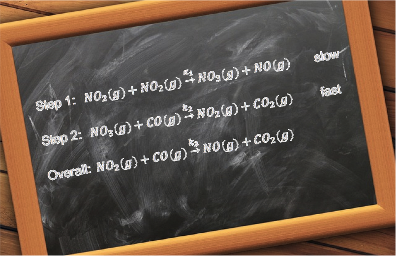
The mechanism of the reaction consists of four steps, each with a particular reaction rate (see diagram below).

The overall rate of reaction is dependent on the slowest step, which is called the rate determining step. As the rate determining step for the above reaction is the rearrangement of the first intermediate CH₃C(OH)CH₃⁺ to the second intermediate CH₃C(OH)CH₂, the proposed rate law is:

$rate=k_2\left [ CH_3C(OH)CH_3^+ \right ]\; \; \; \; \; \; \; \; 43$

However, in chemical kinetics, we are interested in analysing the effect of varying concentrations of reactants on the rate of the reaction. Therefore, we modify eq43 to reflect the concentrations of reactants by noting that

- k₂ « k_-1, such that we assume [CH₃C(OH)CH₃⁺] attains a constant value before the conversion of CH₃C(OH)CH₃⁺ to CH₃C(OH)CH₂ commences.
- The forward and reverse rates for the first step are equal at equilibrium and hence:

$k_1[CH_3COCH_3][H^+]=k_{-1}[CH_3C(OH)CH_3^{\; \: +}]$

$[CH_3C(OH)CH_3^{\; \: +}]=\frac{k_1}{k_{-1}}[CH_3COCH_3][H^+]\; \; \; \; \; \; \; \; 44$

Substitute eq44 in eq43

$rate=k[CH_3COCH_3][H^+]\; \; \; \; \; where\; \; k=\frac{k_1k_2}{k_{-1}}$

which is eq42.

An energy profile diagram of this reaction (see diagram above) shows four activated complexes with energies coinciding with the peaks (denoted by green dots) and three intermediates with potential energies matching the three troughs of the curve (denoted by red dots). It is important to note that an intermediate is a relative stable and isolable chemical species that exists for a finite time, while an activated complex is an unstable, non-isolable chemical structure that has only a transient existence.

Question

Propose a two-step mechanism for the reaction $2NO+O_2\rightarrow 2NO_2$ , which has the experimentally observed rate law: $rate=k[NO]^2[O_2]$ .

Answer

The rate determining step must involve O₂ or NO or both. Let’s suppose it is the final step of the mechanism and has O₂ as a reactant:

$M+O_2\; \; \begin{matrix} k_2\\\rightarrow \end{matrix}\; \; 2NO_2$

where M is an unknown intermediate molecule.

This implies that the preceding step is possibly:

$2NO\; \begin{matrix} k_1\\\rightleftharpoons \\ k_{-1} \end{matrix}\; M$

Balancing the above equations reveals the intermediate as: N₂O₂ . To check whether the proposed mechanism is reasonable, we write the rate law for the rate determining step:

$rate=k_2[N_2O_2][O_2]\; \; \; \; \; \; \; \; 45$

If we assume k₂ « k_-1 such that [N₂O₂] attains a constant value before it reacts with O₂, we can substitute the equilibrium expression of $k_1[NO][NO]=k_{-1}[N_2O_2]$ in eq45 to give:

$rate=k[NO]^2[O_2]\; \; \; \; \; where\; k=\frac{k_1k_2}{k_{-1}}$

To further validate the proposed mechanism, we need to isolate the intermediate.

Next article: Iodine clock

Previous article: Arrhenius equation

Content page of intermediate chemical kinetics

Content page of intermediate chemistry

Main content page

November 4, 2019November 20, 2025

Iodine clock experiment (chemical kinetics)

A typical iodine clock experiment seeks to determine the rate law of a reaction.

For the peroxide-iodide reaction $H_2O_2+2H^++2I^-\rightarrow 2H_2O+I_2$ , a proposed rate law is:

$rate=k[H_2O_2]^x[H^+]^y[I^-]^z\; \; \; \; \; \; \; \; 48$

Since the rate of the peroxide-iodide reaction is relatively slow, the method of initial rates can be used to determine the rate law. Let’s suppose a series of peroxide-iodide experiments is conducted at room temperature with the following parameters:

Experiment	Flask 1			Flask 2
Experiment	0.040M H₂O₂/cm³	0.05M H₂SO₄/cm³	Starch/ drops	0.010M KI /cm³	0.001M Na₂S₂O₃/cm³	H₂O/cm³
1	10	10	3	10	10	10
2	10	10	3	20	10	–
3	20	10	3	10	10	–
4	10	20	3	10	10	–

Water is added to experiment 1 so that all four experiments are conducted under the same constant volume. For every experiment, a stopwatch is turned on once the contents of the two flasks are mixed together and turned off when the mixture turns blue-black.

$H_2O_2+2H^++2I^-\rightarrow 2H_2O+I_2\; \; \; \; \; \; \; \; 49$

$2S_2O_3^{\; \: 2-}+I_2\rightarrow S_4O_6^{\; \: 2-}+2I^-\; \; \; \; \; \; \; \; 50$

When the mixture turns blue-black, the initial amount of 1.0×10^-5 moles of thiosulphate in each experiment has reacted with 5.0×10^-6 moles of iodine (eq50), which in turn required 1.0×10^-5 moles of iodide to produce (eq49). This means that we are measuring the time for a constant amount of 5.0×10^-6 moles of iodine to form in each experiment. Hence, we can rewrite eq48 as:

$\frac{d[I_2]}{dt}=\frac{\frac{n_{I_{2,f}}}{V}-\frac{n_{I_2,i}}{V}}{t_f-t_i}=k[H_2O_2]^x[H^+]^y[I^-]^z$

Since $n_{I_2,f}=5.0\times10^{-6}\: moles$ , $n_{I_2,i}=0$ , $V\approx0.05\, dm^3$ , and $t_i=0$

$\frac{\frac{5.0\times10^{-6}}{0.05}}{t_f}=k[H_2O_2]^x[H^+]^y[I^-]^z\; \; \; \; \; \; \; \; 51$

Comparing eq51 and eq48, $rate\propto\frac{1}{t_f}$ . Let’s assume that the experiment is completed with the different times $t_f$ recorded in the table below:

Experiment	Flask 1			Flask 2			Time (t_f)/s	(1/t_f)/10^-2 s^-1
Experiment	0.040M H₂O₂/cm³	0.05M H₂SO₄/cm³	Starch/ drops	0.010M KI /cm³	0.001M Na₂S₂O₃/cm³	H₂O/cm³	Time (t_f)/s	(1/t_f)/10^-2 s^-1
1	10	10	3	10	10	10	21.5	4.65
2	10	10	3	20	10	–	11.2	8.93
3	20	10	3	10	10	–	10.4	9.62
4	10	20	3	10	10	–	22.3	9.18

Comparing experiments 1 and 2, doubling the concentration of KI increases the reaction’s initial rate by $\frac{8.93}{4.65}=1.92$ or approximately two fold. From experiments 1 and 3, doubling the concentration of H₂O₂ increases the reaction’s initial rate by $\frac{9.62}{4.65}=2.07$ or approximately two fold. With reference to experiments 1 and 4, doubling the concentration of the acid increases the initial rate of the reaction by $\frac{9.17}{4.65}=1.97$ or approximately two fold. Notice that the factor, $\frac{5.0\times10^{-6}}{0.05}$ , disappears when we divide $\frac{\frac{5.0\times10^{-6}}{0.05}}{t_f}$ from different experiments to compare the initial reaction rates. Therefore, we use $\frac{1}{t_f}$ instead of $\frac{\frac{5.0\times10^{-6}}{0.05}}{t_f}$ to represent the initial reaction rates and conclude that the rate law is first order with respect to each reactant:

$rate=k[H_2O_2][H^+][I^-]$

NExt article: Radioactive decay

Previous article: Iodine clock

Content page of intermediate chemical kinetics

Content page of intermediate chemistry

Main content page

October 30, 2019October 11, 2025

Real gases: overview

Real gases deviate from ideal behaviour under high pressure and low temperature, exhibiting complex interactions and properties that are essential for understanding their characteristics in various scientific and industrial applications.

The ideal gas law functions well under conditions when gas particles are regarded as:

1. in constant random motion.
2. point masses with zero volume.
3. very far apart from one another
4. devoid of intermolecular forces of attraction or repulsion.
5. perfectly elastic.

Real gases, however, contain molecules that occupy a certain volume that is not negligible compared to the volume of the reaction vessel. Furthermore, intermolecular forces of attraction and repulsion between real gas molecules can be significant under certain conditions. Therefore, real gases deviate from ideality and require other equations of state to describe.

Next article: Compression factor

Content page of real gases

Content page of intermediate chemistry

Main content page

October 30, 2019January 23, 2025

Compression factor

The compression factor or compressibility factor measures the deviation of the behaviour a real gas from an ideal gas.

Intermolecular forces can be attractive or repulsive. Attractive forces have a longer range (several molecules in length) than repulsive forces.

Question

Why do attractive intermolecular forces have a longer range than repulsive intermolecular forces?

Answer

The difference in range between attractive and repulsive intermolecular forces boils down to the nature of these forces and how they act over distance. Attractive forces like van der Waals forces, dipole-dipole interactions, and hydrogen bonds decrease in strength more gradually with distance. For example, van der Waals forces decrease with the inverse sixth power of the distance between molecules. This means that even when molecules are relatively far apart, these forces can still exert a noticeable influence. Repulsive forces, on the other hand, are much stronger and decrease more rapidly with distance. These forces arise primarily from the overlap of electron clouds, leading to a strong repulsion due to the Pauli exclusion principle. The repulsive force increases exponentially as the distance between molecules decreases, making it significant only at very short distances.

At high pressures (high compression), repulsive forces between gas molecules are more significant than attractive forces, as the molecules occupy a small volume with small separations between them. The volume occupied by the gas is therefore expected to be larger than that for an ideal gas.

At low pressures (low compression), neither force is significant, as the gas molecules occupy a large volume with large separations between them. The gas therefore behaves ideally (i.e. volume occupied by the gas is expected to be the same as that for an ideal gas) and can be described mathematically by the ideal gas law.

At moderate pressures, attractive forces are more significant than repulsive forces, as the molecules are close enough for intermolecular attraction but not close enough for repulsive forces to be effective. The volume occupied by the gas is expected to be smaller than that for an ideal gas.

We can therefore measure the deviation of a real gas from ideality by analysing the ratio:

$Z=\frac{V_m}{V_m^{\: o}}\; \; \; \; \; \; \; \; 1$

where V_mis the molar volume of a gas, and V_m^o is the molar volume of an ideal gas at the same temperature and pressure as the gas of V_m.

We call this ratio, Z, the compression factor (or compressibility factor). The possible values of Z are as follows:

Pressure	Z
Low	1
Moderate	< 1
High	> 1

The diagram below shows the values of Z at different pressures for a few gases at the same temperature.

All gases have Z > 1 at high pressures (over 500 atm), Z < 1 at intermediate pressures (0 atm to 500 atm) and Z = 1 as p → 0. Since $V_m^{\: o}=\frac{RT}{p}$ , eq1 becomes

$pV_m=RTZ\; \; \; \; \; \; \; \; 2$

Eq2 is a simple equation of state that accounts for real gases when Z deviates from 1.

Question

Why is Z > 1 for H₂at intermediate pressures?

Answer

From eq2, Z is a function of temperature T. The diagram above shows a plot of Z for T > 100 K, where Z > 1 for H₂ at intermediate pressures. For T < 100 K, Z < 1 for H₂ at intermediate pressures. To elaborate further, H₂is smaller than the other gas molecules represented in the diagram. Therefore, we would expect repulsive forces between H₂molecules to be significant at higher pressures. In other words, H₂behaves like an ideal gas, with Z ≥ 1, at low and intermediate pressures for T > 100 K.

Next article: Critical constants

Previous article: Overview

Content page of real gases

Content page of intermediate chemistry

Main content page

October 30, 2019September 25, 2024

Critical constants

The critical constants of a real gas describe the conditions for liquefaction of the gas.

Thomas Andrews, an Irish chemist, conducted experiments on the liquefaction of gases in the 1860s and developed the concept of critical constants, which is summarised as follows:-

Consider a gas, Y, confined by a piston in a cylinder. The diagram below shows the pressure of the gas in the cylinder as the piston is pushed to vary the volume at various temperatures with T₁> T₂ > T₃ > T₄ > T₅. Each coloured line, called an isotherm, describes the change in pressure versus the change in molar volume of the gas at a specific temperature.

The isotherms at higher temperatures have smooth curves, while those at lower temperatures consist of horizontal portions. As we compress the gas at point A at temperature T₅, its pressure increases until just to the left of point B, where the gas starts to condense into its liquid form (it exists in both the liquid and gaseous phases with a defined surface separating the two). The system is now at equilibrium, where $Y(g)\rightleftharpoons Y(l)$ . The fact that the gas condenses into a liquid implies that it is a real gas (an ideal gas is devoid of intermolecular interactions).

As we manually compress the system further, more liquid is formed, as the system reacts according to Le Chatelier’s principle: the system counteracts the increase in pressure (decrease in volume) by shifting the position of the equilibrium of $Y(g)\rightleftharpoons Y(l)$ to the right to reduce the pressure, resulting in the pressure of the gas being constant. Hence, the curve from B to C is horizontal and is called a tie line. The pressure corresponding to the tie line is known as the vapour pressure of the liquid atT₅. At point C, all the gas is condensed into liquid with the piston touching the surface of the liquid.

The volume hardly changes when we compress the system further from C to D, as the liquid state of a substance is relatively incompressible. If we repeat the entire compression process at higher temperatures, we find that the width of the tie line shortens, e.g. for T₄, where it reduces to a maximum point (marked X) at T₃. We call this point the critical point of the substance and the isotherm that passes through it, the critical isotherm.

The temperature that produces the critical isotherm is called the critical temperature, T_c, e.g. T_cfor CO₂ is 31.04⁰C. The pressure and molar volume at the critical point is known as the critical pressure, p_c, and critical molar volume, V_c, respectively. p_c, V_c, and T_c are collectively called the critical constants of a substance.

The gas that is described by isotherms at temperatures above T_ccannot be compressed into a liquid regardless of the pressure applied. Due to the high pressure environment at temperatures above T_c, the gas has a density that is closer to that of a liquid and is called a supercritical fluid even though it is by definition a gas.

The density of a supercritical fluid and hence its solubility can be optimised for a particular application by adjusting its pressure. Supercritical CO₂, for example, is used to dissolve and extract caffeine from coffee beans and as a dry-cleaning solvent.

Generally, the regions shaded yellow, blue, pink and grey in the above graph represent the gas phase, the liquid-gas phase, the liquid phase and the supercritical fluid phase respectively.

Lastly, it is important to note that at points B, C, X and all other points on the boundary separating the liquid-gas zone from the other zones, the substance exists only in one phase. For example, at the critical point, the meniscus between the liquid and gas (supercritical fluid) phases disappears, as there is no difference in densities of the liquid and gas (supercritical fluid).

Next article: van der Waal’s equation of state

Previous article: Compression factor

Content page of real gases

Content page of intermediate chemistry

Main content page

October 30, 2019December 5, 2024

van der Waal’s equation of state

Johannes van der Waals, a Dutch physicist, introduced an equation in 1873 called the van der Waals equation to mathematically describe the physical state of a real gas.

This equation is:

$\left [ p+a\left ( \frac{n}{V} \right )^2 \right ]\left ( V-nb \right )=nRT\; \; \; \; \; \; \; \; 3$

where a and b are called the van der Waals coefficients, which are temperature-independent constants specific to each gas.

The equation looks similar to the ideal gas equation except for the pressure and volume factors of $a\left ( \frac{n}{V} \right )^2$ and nb, respectively. To understand how van der Waals’ equation is derived, we need to know how the ideal gas law is conceptualised.

The ideal gas equation, pV = nRT, is derived from the combined experiments of Robert Boyle and Jacques Charles, and a principle developed by Amedeo Avogadro. This means that, for a fixed amount of gas at a relatively high temperature, the product of the experimentally observed values of p and V in the equation is a constant. The equation works reasonably well at low pressures where gases approach ideality. Under such conditions, gas particles can be assumed to be point masses with zero volume and, therefore, have no intermolecular forces of attraction or repulsion between them. In other words, the equation only works when the observed variables of p and V are ‘ideal’:

$p_{ideal}V_{ideal}=nRT\; \; \; \; \; \; \; \; 4$

In reality, gases have finite volumes and repel one another, especially at high pressures. The experimentally observed values of pressures and volumes are actually p_real and V_real. Therefore, for eq4 to work, we have to modify it.

Due to the presence of repulsive forces between real gas molecules at high pressures, the observed volume of a real gas is larger than the volume of its ideal counterpart, that is, V_real > V_ideal. The diagram below shows the volume expansion (from yellow to blue) if the point masses have finite volumes.

Letting the difference in molar volume of a real gas and an ideal gas be b, we have $\frac{V_{real}}{n}-\frac{V_{ideal}}{n}=b$ or

$V_{ideal}=V_{real}-nb\; \; \; \; \; \; \; \; 5$

Substituting eq5 in eq4 and rearranging yields

$V_{real}=\frac{nRT}{p_{ideal}}+nb\; \; \; \; \; \; \; \; 6$

Eq6 predicts that the molar volume of a gas at zero Kelvin is b. Experiments indeed reveal that b has approximately the same value as the molar volume of the solid form or liquid form of the gas near that temperature. On the other hand, the ideal gas law, $V_{ideal}=\frac{nRT}{p_{ideal}}$ , wrongly predicts that the volume of a gas at 0 K is zero.

Next, the pressure that a real gas exerts on the wall of a container is lower than the pressure of its ideal counterpart (p_ideal > p_real), as the molecules of a real gas experience intermolecular forces of attraction that decelerates their motion when they are about to impact the wall of the container. This means that we need to add a pressure shortfall, Δp_real, to the observed real pressure to reflect the ideal pressure that fits eq4:

$p_{ideal}=p_{real}+\Delta p_{real}\; \; \; \; \; \; \; \; 7$

If we perceive the intermolecular force of attraction (i.e., the force that one molecule of gas experiences near the wall of the container) as the attraction between that molecule and the bulk of the gas, the pressure shortfall due to that particular molecule is proportional to the density of the gas:

$\Delta p_{real,\, one\, molecule}=k\left ( \frac{n}{V_{real}} \right )$

Furthermore, the total number of molecules N near the wall of the container is again proportional to the density of the gas:

$N=k'\left ( \frac{n}{V_{real}} \right )$

The total pressure shortfall is therefore:

$\Delta p_{real}=N\Delta p_{real,\, one\, molecule}=k'\left ( \frac{n}{V_{real}} \right )k\left ( \frac{n}{V_{real}} \right )=a\left ( \frac{n}{V_{real}} \right )^2$

where a = k’k is a proportionality constant specific to a particular gas.

Eq7 becomes

$p_{ideal}=p_{real}+a\left ( \frac{n}{V_{real}} \right )^2\; \; \; \; \; \; \; \; 8$

Substituting eq5 and eq8 in eq4, we get the explicit form of eq3:

$\left [ p_{real}+a\left ( \frac{n}{V_{real}} \right )^2 \right ]\left ( V_{real}-nb \right )=nRT\; \; \; \; \; \; \; \; 9$

The pressure and volumes in eq9 now represent experimentally observed real pressure and real volumes, respectively. We have essentially converted an equation that only works for ideal gases into one that is applicable for real gases. For simplicity, we can omit the subscripts, which gives eq3.

Using eq3, the van der Waals equation can also be expressed in the molar form by substituting it with the molar volume, $V_m=\frac{V}{n}$ , to give:

$\left ( p+\frac{a}{V_m^{\: 2}} \right )\left ( V_m-b \right )=RT$

which rearranges to:

$p=\frac{RT}{V_m-b}-\frac{a}{V_m^{\: 2}}\; \; \; \; \; \; \; \; 10$

At high molar volumes (i.e. low pressures), V_m – b ≈ V_m and the second term on the RHS of eq10 becomes very small, with eq10 reducing to the ideal gas equation: $p\approx \frac{RT}{V_m}$ .

The van der Waals equation is an improvement over eq2, as it is able to describe the physical state of a real gas in terms of the van der Waals coefficients a and b, which relate to the strength of the forces of attraction between molecules and the size of the molecules, respectively.

Since the critical isotherm of a gas has an inflexion point at the critical point, we can determine the van der Waals coefficients for a gas by finding the 1^st and 2^nd derivatives of eq10, letting these be equal to zero and solving for the critical constants:

$\frac{dp}{dV_m}=-\frac{RT}{\left ( V_m-b \right )^2}+\frac{2a}{V_m^{\: 3}}=0\; \; \; \; \; \; \; \; 11$

$\frac{dp}{dV_m}=\frac{2RT}{\left ( V_m-b \right )^3}-\frac{6a}{V_m^{\:4}}=0\; \; \; \; \; \; \; \; 12$

From eq11 and eq12, $a=\frac{RTV_c^{\: 3}}{2\left ( V_c-b \right )^2}$ and $a=\frac{RTV_c^{\: 4}}{3\left ( V_c-b \right )^3}$ respectively. Combining both values of a,

$V_c=3b\; \; \; \; \; \; \; \; 13$

Substitute eq13 back in eq11 where V_m is now V_c,

$T_c=\frac{8a}{27Rb}\; \; \; \; \; \; \; \; 14$

Substitute eq13 and eq14 back in eq10,

$p_c=\frac{a}{27b^2}\; \; \; \; \; \; \; \; 15$

Hence, by measuring the pressure, volume and temperature at the critical point of a gas (i.e. the critical constants), we can calculate the van der Waals coefficients for that gas. The table below shows the van der Waals coefficients for some common gases:

	a / atm dm⁶mol^-2	b / 10^-2 dm³mol^-1
H₂	0.2420	2.65
N₂	1.352	3.87
O₂	1.364	3.19
CO₂	3.610	4.29

Question

Answer

Next article: Arrhenius equation

Previous article: Why is Initial rate proportional to 1/t?

Question

Answer

Next article: Isolation method

Previous article: Initial rate method

Question

Answer

Next article: REaction mechanism

Previous article: Isolation method

Next article: Iodine clock experiment

Previous article: Reaction mechanism

Question

Answer

Next article: Iodine clock

Previous article: Arrhenius equation

NExt article: Radioactive decay

Previous article: Iodine clock

Next article: Compression factor

Question

Answer

Question

Answer

Next article: Critical constants

Previous article: Overview

Next article: van der Waal’s equation of state

Previous article: Compression factor

Next article: Virial equation of state

Previous article: Critical constants