The degenerate perturbation theory, an extension of the perturbation theory, is used to find an approximate solution to a quantum-mechanical problem involving non-perturbed states that are degenerate.
In the non-degenerate case, it is unambiguous that , i.e.
is described by individual basis states
. However, for a set of degenerate orthonormal states
(
denotes the same eigenvalue for all states in the set) of the unperturbed Hamiltonian
, where
,
can represent any linear combination of
or the non-degenerate states
, where
. If there are more than one set of degenerate states, each set with a distinct energy level,
represents linear combinations of
, linear combinations of
, and so on, and individual states of
, where
.
For each set of degenerate orthonormal states, e.g. , of the unperturbed Hamiltonian
, the linear combination
(where
is the degeneracy) is an eigenstate of
with the same eigenvalue
:
Therefore, the derivation in the previous article branches off from eq267. While is no longer unambiguously described by individual basis states
,
is still
. So, eq267 becomes
Multiplying the above equation from the left by and integrating,
When , we have.
Since represents the matrix elements of
, eq273 implies that in the presence of degenerate states, the first-order perturbation theory only works if we can select appropriate wavefunctions that diagonalise
.
Consider the case of just one set of degenerate orthonormal states of the unperturbed Hamiltonian
, with the other states of
being non-degenerate. If we further analyse the subspace of
, we substitute
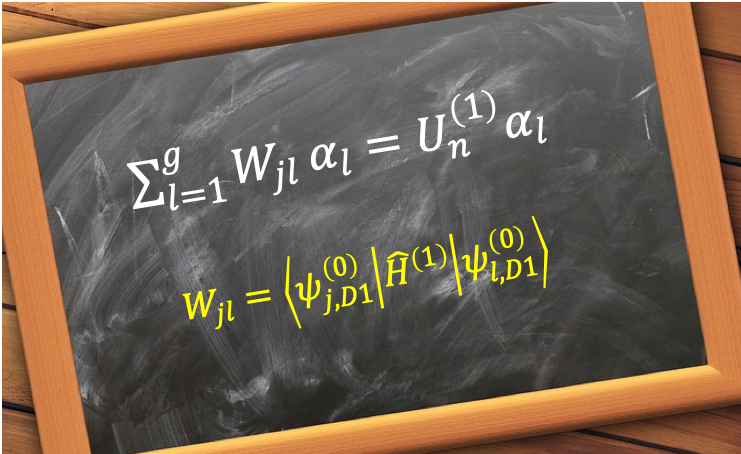
in eq272 to give:
Taking the inner product with and using eq36 on the first term,
where are the matrix elements of
.
Rewriting the eigenvalue equation of eq274 in matrix form,
where is the
identity matrix.
Eq275 is a linear homogeneous equation, which has non-trivial solutions if
Expanding the determinant (also known as a secular equation), we get the characteristic equation, which can be solved for the roots of . Each of these roots is then substituted into eq274 to find the set of coefficients
and hence, the exact eigenstates
. If these exact eigenstates diagonalises
, we refer to them as “good” states, which allow
to be calculated (see next article for an example).

Question
What is a linear homogeneous equation? Why does a linear homogeneous equation have non-trivial solutions if the determinant of the operator is zero?
Answer
A linear homogeneous equation is a matrix equation of the form , where
is an
matrix and
is column vector. Let
be a
matrix representing three position vectors and
. We have
So, ,
and
. Now, a non-trivial solution of
occurs when
. Therefore, we require any non-zero position vector
that is orthogonal to
. This is fulfilled if the position vectors
lie in a plane, which happens when the scalar triplet product
(which is equal to the volume of the parallelepiped spanned by
) is zero. Since the scalar triple product is also equal to the determinant of
, i.e.
(which can be easily proven by expanding both sides and showing that LHS equals to RHS),
has non-trivial solutions if
.
Since there are multiple roots of , the perturbation
usually lifts the degeneracy of the unperturbed states. An example is the relativistic Hamiltonian’s spin-orbit coupling perturbation
, which splits terms
into levels
. If there are equal roots, we would need to further analyse the problem with higher order perturbations to completely lift the degeneracy (as is the case when considering the Zeeman effect).
Question
Find the characteristic equation for the degenerate set .
Answer
Eq276 becomes,