Biot-Savart law

The Biot-Savart law is an equation describing the magnetic field generated by a current segment. Consider a point $\small P$ in the vicinity of a wire carrying a current $\small I$ (see diagram below).

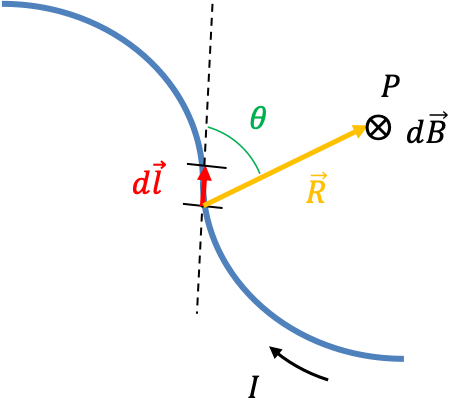
The magnitude of $\small I$ represents the amount of charges flowing through the wire (blue line). This implies that the amount of charges in an infinitesimal length of the wire $\small d\vec{l}$ is proportional to $\small Id\vec{l}$ . Since the magnetic field $\small d\vec{B}$ at $\small P$ is generated by the amount of moving charges in the wire, we have $\small d\vec{B}\propto Id\vec{l}$ , or rather $\small d\vec{B}\propto Id\vec{l}sin\theta$ because $\small d\vec{B}$ is due to component of $\small d\vec{l}$ that is perpendicular to $\vec{R}$ (use right-hand rule to visualise).

The magnetic flux generated by $\small I$ radiates spherically outward from every point along the infinitesimal length of the wire. For a particular $\small I$ in a segment $\small d\vec{l}$ , the amount of magnetic field lines radiated is a constant. As $\small R$ increases, the surface area of the sphere becomes bigger. Therefore, the radiation passing through $\small P$ must be proportional to the unit area of the sphere at $\small R$ , i.e. $\small d\vec{B}\propto \frac{1}{4\pi R^{2}}\hat{R}$ , where $\small \hat{R}$ is the unit vector in the direction of $\small \vec{R}$ . Finally, we would expect $\small d\vec{B}$ to vary according to the material of the wire and the medium of the space between the wire and $\small P$ . If we assume the wire to have negligible resistance and that the system is in a vacuum, we have

$\small d\vec{B}=\frac{\mu_0Id\vec{l}sin\theta\hat{R}}{4\pi R^{2}}=\frac{\mu_0Id\vec{l}sin\theta\vec{R}}{4\pi R^{3}}=\frac{\mu_0Id\vec{l}\times\vec{R}}{4\pi R^{3}}\; \; \; \; \; \; \; \; 150$

where $\small \mu_0$ is called the vacuum permeability or magnetic permeability of free space, and it represents the proportionality constant for the measurement of $\small d\vec{B}$ at $\small P$ in a vacuum.

The scalar form of eq150 is

$\small d\vec{B}=\frac{\mu_0Idlsin\theta}{4\pi R^{2}}\; \; \; \; \; \; \; \; 151$

The total field at $\small P$ is

$\small \vec{B}=\frac{\mu_0}{4\pi}\int \frac{Id\vec{l}\times\vec{R}}{R^{3}}\; \; \; \; \; \; \; \; 152$

Eq150, eq151 and eq152 are different forms of the Biot-Savart law.

If the wire is a circle, the direction of $\small d\vec{B}$ at $\small P$ is determined by the right hand rule and is perpendicular to the plane formed by $\small d\vec{l}$ and $\small \vec{R}$ , where the angle $\small \theta$ between $\small d\vec{l}$ and $\small \vec{R}$ is $\small 90^{\circ}$ (see diagram below).

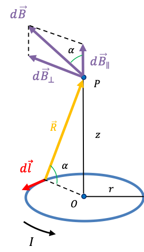
From eq151,

$\small dB=\frac{\mu_0Idlsin90^{\circ}}{4\pi R^{2}}=\frac{\mu_0Idl}{4\pi R^{2}}\; \; \; \; \; \; \; \; 153$

Let’s analyse the components of $\small d\vec{B}$ . If we sum all the vectors of $\small d\vec{B}_\perp$ at $\small P$ from all current elements around the wire, they cancel out. The vectors of $\small d\vec{B}_\parallel$ at $\small P$ , however adds. Therefore, in scalar form, $\small B=\int dB_\parallel$ , where $\small dB_\parallel=dBcos\alpha$ , which when combined with eq153 gives

$\small dB_\parallel=\frac{\mu_0Icos\alpha}{4\pi R^{2}}dl\; \; \; \; \; \; \; \; 154$

Since $\small R=\sqrt{r^{2}+z^{2}}$ and $\small cos\alpha=\frac{r}{\sqrt{r^{2}+z^{2}}}$ , eq154 becomes $\small dB_\parallel=\frac{\mu_0Ir}{4\pi(r^{2}+z^{2})^{3/2}}dl$ and

$\small B=\int dB_\parallel=\frac{\mu_0Ir}{4\pi(r^{2}+z^{2})^{3/2}}\int dl$

Substituting $\small \int dl=2\pi r$ in the above equation

$\small B=\frac{\mu_0Ir^{2}}{2(r^{2}+z^{2})^{3/2}}\; \; \; \; \; \; \; \; 155$

For the case of $\small B$ at point $\small O$ , we have $\small z$ , which is the length $\small OP$ , equals to zero. So,

$\small B=\frac{\mu_0I}{2r}\; \; \; \; \; \; \; \; 156$

For the case of $\small z\gg r$ , eq155 becomes $\small B=\frac{\mu_0IA}{2\pi z^{3}}$ , where $\small A=\pi r^{2}$ . Substitute eq60 and eq61 in $\small B$ ,