Intermediate Chemistry - Mono Mole

December 18, 2018October 22, 2025

Classical atomic theory

The classical atomic theory is an early scientific interpretation of the atom.

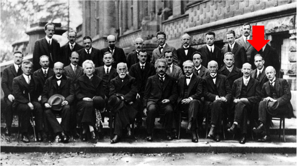
Niels Bohr, a Danish physicist, introduced a model in 1911 to explain the hydrogen spectrum, which he used to derive the Rydberg formula.

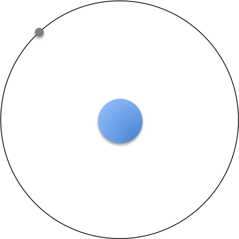
He proposed that the electron of a hydrogen atom orbits around the fixed massive nucleus (see diagram below), with the coulombic force of interaction between the electron and the nucleus being balanced by the centrifugal force; that is:

$\frac{e^2}{4\pi \varepsilon _0r^2}=\frac{m_ev^2}{r}\; \; \; \; \; \; \; \; 1$

where e is the charge on the electron, ε₀is permittivity of free space, r is the radius of the orbit, m_e is the mass of the electron, and v is the speed of the electron.

Bohr further proposed that, for an orbit to remain stable, the angular momentum of the electron must be an integer multiple of $\hbar=h/2\pi$ :

$m_evr=n\frac{h}{2\pi}\; \; \; \; \; \; \; \; 2$

where $h$ is the Planck constant.

Combining eq1 and eq2 and eliminating $v$ yields

$r=\frac{\varepsilon _0n^2h^2}{\pi m_ee^2}\; \; \; \; \; \; \; \; 3$

Substituting eq3 back in eq2 gives

$v=\frac{e^2}{2\varepsilon _0nh}\; \; \; \; \; \; \; \; 4$

Question

What is angular momentum and how did Bohr arrive at the assumption for eq2?

Answer

Angular momentum is the rotational analogue of linear momentum. While the momentum of a body travelling in a straight line is proportional to its mass and velocity (p = mv), the momentum of a body revolving around a point is proportional to its mass, tangential velocity, and the perpendicular distance from its tangential velocity to the point (L = mvr). According to Bohr, electrons orbit the nucleus at distinct radii and, consequently, have discrete values of angular momentum. He proposed that these radii are such that the angular momentum are integer multiples of $h/2\pi$ .

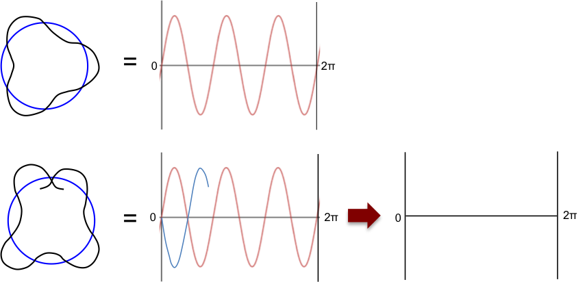
Louis de Broglie, a French physicist, subsequently reinterpreted Bohr’s model by treating electrons as waves. He proposed that an integral number of the electron’s wavelength $\lambda$ must fit the orbit’s circumference for the orbit to be stable, i.e. $2\pi r=n\lambda$ , where $n\in \mathbb{Z}$ . Otherwise, the orbiting wave will disappear due to destructive interference (see diagram below).

Substituting de Broglie’s formula of p = h/λ into 2πr = nλ gives

$p=\frac{nh}{2\pi r}\; \; \; \Rightarrow \; \; \; v=\frac{nh}{2\pi rm_e}\; \; \; and\; \; \; r=\frac{nh}{2\pi vm_e}\; \; \; \; \; \; \; (5)$

Substituting eq5 in eq1 yields

$v=\frac{e^2}{2\varepsilon _0nh}\; \; \; and\; \; \; r=\frac{\varepsilon _0 n^2h^2}{\pi m_ee^2}\; \; \; \; \; \; \; (6)$

which is the same as eq4 and eq3, respectively.

The total energy of the electron is:

$E_n=KE+V=\frac{1}{2}m_ev^2-\frac{e^2}{4\pi \varepsilon _0r}\; \; \; \; \; \; \; (7)$

Substituting eq3 and eq4 in eq7 results in

$E_n=-\frac{m_ee^4}{8{\varepsilon _{0}}^{2}n^2h^2}\; \; \; \; \; \; \; (8)$

The transition energy between two states is:

$\Delta E=E_2-E_1=\frac{m_ee^4}{8{\varepsilon _{0}}^{2}h^2}(\frac{1}{{n_{1}}^{2}}-\frac{1}{{n_{2}}^{2}})\; \; \; \; \; \; \; (9)$

At this point, Bohr assumed that an allowed transition between two states involves an electron falling from a higher energy state to a lower energy state, with the emission of a photon of energy given by the Planck relation E_p= hv = ΔE. Therefore, eq9 becomes:

$hv=hc\tilde{v}=\frac{m_ee^4}{8{\varepsilon _{0}}^{2}h^2}(\frac{1}{{n_{1}}^{2}}-\frac{1}{{n_{2}}^{2}})$

$\tilde{v}=\frac{m_ee^4}{8{\varepsilon _{0}}^{2}ch^3}(\frac{1}{{n_{1}}^{2}}-\frac{1}{{n_{2}}^{2}})\; \; \; \; \; \; \; (10)$

where $\tilde{v}=\frac{1}{\lambda}$ is the wavenumber of the photon.

When n₁= 1 and n₂= ∞,

$\tilde{v}=\frac{m_ee^4}{8{\varepsilon _{0}}^{2}ch^3}=R_H\;\; or\; \; R_\infty \; \; \; \; \; \; \; (11)$

where R_Hor R∞is the Rydberg constant.

Even though the Bohr model has certain shortcomings – specifically, that an electron orbiting around the nucleus would constantly radiate electromagnetic energy and eventually crash into the nucleus – eq10 and eq11 were proven to be mathematically sound for the hydrogen atom using quantum mechanics.

From eq11,

$m_e=\frac{8{\varepsilon _{0}}^{2}ch^3R_\infty }{e^4}=\frac{2hR_\infty }{c\alpha ^2}\; \; \; \; \; \; \; (12)$

where $\alpha =\frac{e^2}{2\varepsilon _0hc}\; \; or\; \; \frac{e^2}{4\pi \varepsilon_0\hbar c}\; \; \; \; \; \; \; \; (\hbar=\frac{h}{2\pi})$

$\alpha$ is known as the fine-structure constant.

Question

Show that the molar mass of carbon-12, M(¹²C), is:

$M(^{12}C)=\frac{24hR_\infty N_A}{c\alpha ^2A_r(e)}$

Answer

$\frac{molar\; mass\; of\; ^{12}C}{molar\; mass\; of\; electron}=\frac{relative\; mass\;of\; ^{12}C}{relative \; mass\; of\; electron}$

Since the relative mass of ¹²C is 12 unified atomic mass units,

$\frac{M(^{12}C)}{M(e)}=\frac{12}{A_r(e)}$

From eq12, $M(e)=\frac{2hR_\infty }{c\alpha ^2}N_A$ . Therefore,

$M(^{12}C)=\frac{24hR_\infty N_A}{c\alpha ^2A_r(e)}$

Next article: modern atomic structure

Content page of intermediate quantum chemistry

Content page of intermediate chemistry

Main content page

December 17, 2018July 13, 2025

Link between unified atomic mass and inertia mass

What is the link between unified atomic mass unit and inertia mass?

Jean Perrin’s and other scientists’ experiments in the early 1900s to determine the Avogadro constant were based on a gramme-molecule, which is the mass of a gas that occupies the same volume as two grammes of hydrogen gas at the same temperature and pressure. Their experiments produced a range of values for the constant when different gases are used. This variation occurs because different real gases with the same number of particles have different volumes.

A better definition of the mole was therefore needed and was established in 1967 as follows:

The amount of substance of a system that contains as many elementary entities as there are atoms in 0.012 kilogram of carbon-12.

The choice to base the Avogadro constant on carbon-12 may seem arbitrary. However, it is this definition that enables us to link the unified atomic mass unit scale to the inertia mass scale. So,

$1^{12}C=12u$

$\frac{0.012\; kgmol^{-1}}{N_{A}\; mol^{-1}}=12u\; \; \; \; \; \; \; (1)$

$1u=1.660539\times 10^{-27}\; kg\; \; \; \; \; \; \; (2)$

We can rewrite eq1 as

$1u=\frac{M_{u}}{N_{A}}g$

where M_uis the molar mass constant and is equal to 1 gmol^-1.

Even though the definition of the mole was changed to ‘a mole is the amount of substance of a system that contains exactly 6.02214076 x 10²³ elementary entities’ in Nov 2018, the peg of 1¹²C to 12 u remains. However, the exact value of the Avogadro constant leads to the molar mass of carbon-12 having a relative uncertainty in the order of 10^-10. It is no longer exactly 0.012 kgmol^-1 and is given by the formula (see the article on ‘Bohr model‘ for derivation):

$M(^{12}C)=\frac{24hR_{\infty }N_{A}}{c\alpha^{2}A_{r}(e)}\; \; \; \; \; \; \; \; (3)$

where

$h$ is the Planck constant

$R_{\infty }$ is the Rydberg constant

$c$ is the speed of light

$\alpha$ is the fine-structure constant

$A_{r}(e)$ is the ‘relative atomic mass’ of an electron

The uncertainty in the value of 0.012 kgmol^-1, which will be determined in future experiments, is primarily due to the uncertainty in the fine-structure constant.

Similarly, the molar mass constant , which was a constant with the value 1 gmol^-1, is now described by the formula:

$M_{u}=\frac{2hR_{\infty}N_{A}}{c\alpha ^{2}A_{r}(e)}$

By the same logic, the unified atomic mass unit has the formula:

$u=\frac{2hR_{\infty }}{c\alpha^{2}A_{r}(e)}$

next article: how to ‘weigh’ an atom?

previous article: unified atomic mass unit

Content page of mass in chemistry

Content page of intermediate chemistry

Main content page

December 13, 2018October 17, 2024

Millikan’s oil drop experiment: overview

Robert Millikan conducted an experiment in 1909 to measure the charge of an electron. He devised an apparatus to observe electrically-charged droplets of oil between two horizontal plates that had a potential difference of several thousand volts applied across them.

The oil droplets were sprayed from an atomiser into an upper chamber. In the space between the plates, the air were ionised by X-rays, causing the oil droplets to acquire electrons and become negatively charged as they fell and traversed through the air between the plates. Millikan then performed a few tasks and observed the motion of the oil droplets through a microscope.

Next ArTicle: Task 1

Content page of millikan’s oil drop experiment

Content page of intermediate chemistry

Main content page

December 13, 2018October 17, 2024

Millikan’s oil drop experiment: task 1

Millikan’s oil drop experiment consists of a few tasks.

For a start, the power supply to the plates is cut off (V = 0). The oil-droplets falling between the plates accelerate due to the effect of gravitational force and then continue downwards at terminal velocity as they encounter increasing air resistance. The three forces acting on an oil droplet are:

Gravitational force,

F_g

The force of attraction between the mass of the earth and that of the oil droplet.

Upthrust (buoyant),

F_u

The force exerted by a liquid or a gas on a body when the body displaces some weight of the liquid or gas. It is due to the pressure difference between the top and bottom of the object (as a result of the collision of liquid or gas molecules with the body from the top and bottom) and equal to the weight of the liquid or gas displaced.

Drag (viscous),

F_d

The force caused by relative motion (friction) between an object and a liquid or gas. It is proportional to the velocity of the object, the radius of the object and the viscosity of the liquid or gas.

At terminal velocity,

$F_{g}=F_{d}+F_{u}\; \; \; \; \; \; \; (1)$

The oil droplet is assumed to be spherical. So, F_g, the weight of the oil droplet, is:

$F_{g}=mg=\frac{4\pi }{3}r^{3}\rho g\; \; \; \; \; \; \; (2)$

where m, ρ and r are the mass, density and radius of the oil droplet, respectively.

The equation of the drag force acting on the oil droplet can be expressed using Stokes’ law:

$F_{d}=6\pi r\eta v_{1}\; \; \; \; \; \; \; (3)$

where v₁, is the terminal velocity of the falling oil droplet and η is the viscosity of air.

Through the microscope, Millikan recorded the distance travelled by the falling oil droplet over a period of time and calculated the terminal velocity v₁.

For a perfectly spherical oil droplet the upthrust acting on it is:

$F_{u}=mg=\frac{4\pi }{3}r^{3}\rho _{air}g\; \; \; \; \; \; \; (4)$

where ρ_air is the density of the air.

Substituting eq2, eq3 and eq4 in eq1 yields

$6\pi r\eta v_{1}=\frac{4\pi }{3}r^{3}(\rho -\rho _{air})g\; \; \; \; \; \; \; (5)$

$r=\sqrt{\frac{9\eta v_{1}}{2g(\rho -\rho _{air})}}\; \; \; \; \; \; \; (6)$

NEXT ARTICLE: TASK 2

Previous article: Overview

Content page of millikan’s oil drop experiment

Content page of intermediate chemistry

Main content page

December 13, 2018October 17, 2024

Millikan’s oil drop experiment: task 2

The power supply to the plates is turned back on and the electric force acting on the oil droplet is:

$F_{e}=qE\; \; \; \; \; \; \; (7)$

where q is the charge on the oil droplet and E is the electric field between the plates.

For parallel plates,

$E=\frac{V}{d}\; \; \; \; \; \; \; (8)$

where V is the potential difference across the plates and d is the distance between the plates.

Combining eq7 and eq8,

$q=\frac{F_{e}\: d}{V}\; \; \; \; \; \; \; (9)$

If V is adjusted until the oil droplet remained stationary,

$F_{e}=mg\; \; \; \; \; \; \; (10)$

Combining eq9 and eq10,

$q=\frac{mgd}{V}$

Our objective is to determine the value of q, but it is difficult to accurately measure m. Therefore, we have to carry out another task.

NEXT ARTICLE: TASK 3

Previous article: task 1

Content page of millikan’s oil drop experiment

Content page of intermediate chemistry

Main content page

December 13, 2018October 17, 2024

Millikan’s oil drop experiment: task 3

Next, V is turned up slightly so that the oil droplet rises with a new terminal velocity v₂.

We have:

$F_{e}+F_{u}=F_{d}+F_{g}\; \; \; \; \; \; \; (11)$

Note that the electric force is acting upwards (since the oil droplet is rising); upthrust is also acting upwards (because the pressure is still greater below the object than above it due to the exponential distribution of air); drag is now acting downwards because the oil droplet is rising, and weight continues to act downwards due to the effect of gravitational force. Substituting eq2, eq3 (with v₂instead of v₁), eq4 and eq7 in eq 11 yields

$qE+\frac{4\pi }{3}r^{3}\rho _{air}g=6\pi \eta rv_{2}+\frac{4\pi }{3}r^{3}\rho g$

$qE-\frac{4\pi }{3}r^3(\rho -\rho _{air})g=6\pi \eta rv_{2}\; \; \; \; \; \; \; (12)$

Substituting eq5 in eq12 gives

$qE-6\pi r\eta v_{1}=6\pi \eta rv_{2}\; \; \; \; \; \; \; (13)$

Substituting eq8 in eq13 and rearranging results in

$q=\frac{6\pi r\eta (v_{1}+v_{2})d}{V}\; \; \; \; \; \; \; (14)$

Once again, Millikan recorded the distance travelled by the rising oil droplet over a period of time and calculated the new terminal velocity, v₂.

Substituting the values of v₁, v₂and the calculated value of r (from eq6) in eq14, Millikan determined a value for q. He repeated the experiment multiple times, each time varying the strength of X-rays ionizing the air, resulting in a varying number of electrons attaching to the oil droplet. He then obtained various values of q and found them to be multiples of 1.5924 x 10^-19C. Millikan concluded that the value of 1.5924 x 10^-19C is equal to the charge of a single electron. Subsequent determinations refined that value to 1.602176487 x 10⁻¹⁹ C.

Using the Faraday constant and the value of the charge of a single electron that he determined, Millikan calculated the Avogadro constant and proved that one Faraday is the quantity of charge for one mole of electrons.

Previous article: task 2

Content page of millikan’s oil drop experiment

Content page of intermediate chemistry

Main content page

December 13, 2018February 25, 2026

Mass spectrometry: the mechanics

Mass spectrometry in the early days focuses on determining the charge-to-mass ratio, e/m, of an electron. This involves a few steps, beginning with the electric field turned on and the magnetic field turned off. The diagram below shows the mechanics of the electrons as they pass through the electric field plates.

An electric force, F_e, acts on an electron with charge, e, passing through the electric field, E, in the x-direction where

$F_{e}=eE\; \; \; \; \; \; \; (1)$

and gives the electron with mass, m, an acceleration, a:

$F_{e}=ma\; \; \; \; \; \; \; (2)$

Combining eq1 and eq2,

$a=\frac{eE}{m}\; \; \; \; \; \; \; (3)$

As the electric force acts only in the y-direction, the velocity of the electron in the x-direction remains constant at v_H. The velocity of the electron in the y-direction, v_V, is zero at the point where it enters the electric field and increases to a maximum value at the point where the electron leaves the electric field. This maximum value of v_Vremains constant after the electron exits the electric field and is given by:

$v_{V}=\frac{dS}{dt}=\frac{d(ut+\frac{1}{2}at^{2})}{dt}=at$

where S is the displacement of the electron in the y-direction, u is the initial velocity of the electron in the y-direction before entering the electric field (i.e. u = 0) and t is the time during which the electric force acts on the electron.

In other words, t is the time taken for the electron to travel the length of the electric field plate, L. Therefore,

$v_{V}=at=(\frac{eE}{m})(\frac{L}{v_{H}})\; \; \; \; \; \; \; (4)$

The trigonometric relationship between v_H and v_V after the electron leaves the electric field is:

$tan\theta =\frac{v_{V}}{v_{H}}=\frac{eEL}{{v_{H}}^{2}m}\; \; \; \; \; \; \; (5)$

The electric field strength is adjusted so that the angle of deflection is small. Therefore, tanθ ≈ θ and eq5 becomes,

$\theta =\frac{eEL}{{v_{H}}^{2}m}\; \; \; \; \; \; \; (6)$

The value of θ is recorded, leaving v_H as the only unknown variable (in eq6) for the calculation of e/m. To determine v_H , the magnetic field, B, is turned on while the electric field is still on. Using Fleming’s left hand rule, the magnetic force, F_B, acts on the electron (at the point when the electron just enters the magnetic field from the left side) and deflects it in the negative y-direction:

$F_B=ev_HB\; \; \; \; \; \; \; \; (7)$

The magnetic field is then adjusted to the extent that the angle of deflection of the cathode ray is zero, meaning F_e= F_B. Substituting eq1 and eq7 in F_e= F_B, we have:

$v_{H}=\frac{E}{B}\; \; \; \; \; \; \; (8)$

Substitute eq8 in eq6

$\frac{e}{m}=\frac{E\theta }{B^{2}L}\; \; \; \; \; \; \; (9)$

The values of all the variables on the right hand side of eq9 are now known and the charge-to-mass ratio e/m of the electron can be determined. The magnitude of e/m that Thomson obtained ranged from 0.7 x 10¹¹ C/kg to 2 x 10¹¹ C/kg. The currently accepted value is 1.758820024 x 10¹¹ C/kg.

Finally, in 1909, when Robert Millikan determined the charge of an electron via his famous oil drop experiment, the estimated mass of an electron was calculated.

next article: application, relative isotopic mass

Previous ArTicle: J.J. thomson’s cathode ray experiment

Content page of mass spectrometry

Content page of intermediate chemistry

Main content page

December 13, 2018September 25, 2024

Application of mass spectrometry: relative isotopic mass

A mass spectrometer measures the mass of an isotope relative to that of carbon-12 by analysing the ratio of the ionised isotope’s deflection to the ionised carbon-12’s deflection.

From eq9, we have:

$\frac{e_{isotope}}{m_{isotope}}=\frac{E\theta _{isotope}}{B^{2}L}\; \; \; \; \; \; \; (10)$

$\frac{e_{^{12}C}}{m_{^{12}C}}=\frac{E\theta _{^{12}C}}{B^{2}L}\; \; \; \; \; \; \; (11)$

Assume both ions are univalent so that $e_{^{12}C}=e_{isotope}$ and divide eq11 by eq10:

$\frac{m_{isotope}}{m_{^{12}C}}=\frac{\theta _{^{12}C}}{\theta _{isotope}}\; \; \; \; \; \; \; (12)$

Therefore,

$mass\; of\; isotope=\frac{\theta _{^{12}C}}{\theta _{isotope}}m_{^{12}C}\; \; \; \; \; \; \; (13)$

We can also represent eq13 in the form

$mass\; of\; isotope=\frac{m_{isotope}/z_{isotope}}{m_{^{12}C}/z_{^{12}C}}m_{^{12}C}\; \; \; \; \; \; \; (14)$

where we have replaced e with the notation z. The output of eq14 is a value with unit of unified atomic mass unit, u, since the ratio is unit-less while $m_{^{12}C}=12u$ .

Finally, we divide the output of eq14 by 1u to obtain the relative isotopic mass, which is a dimensionless quantity that is defined as the ratio of the mass of an isotope in unified atomic mass unit to one unified atomic mass unit.

Question

Is it possible to accurately measure the mass of an atom in kg using eq9 without a reference isotope?

Answer

No. Due to the limits of precision engineering, measurements of the mass of an atom in kg by directly applying eq9 differ from one mass spectrometer to another. We therefore need a reference ‘flight path’ that we can compare with, i.e. using eq14. Since the value of $m_{^{12}C}$ is accurately defined in u, the output of eq19 must be in unified atomic mass unit. The value in kg is then obtained by the following conversion:

1u = 1.660539 x 10^-27 kg

Next ArTicle: Modern mass spectrometer design

Previous ArTicle: the mechanics

Content page of Mass spectrometry

Content page of intermediate chemistry

Main content page

December 13, 2018October 27, 2024

J. J. Thomson’s cathode ray experiment

Mass spectrometry is an analytical technique that utilises an instrument called a mass spectrometer to identify and quantify ions based on their mass-to-charge ratios. J. J. Thomson, an English physicist, constructed one of the earliest mass spectrometers (see diagram below) and demonstrated in an experiment in 1897 that atoms are made of subatomic particles called electrons. Using the spectrometer, he determined the charge-to-mass ratio of an electron.

The ioniser on the left of the spectrometer is not a complete vacuum; it is filled with a trace amount of air molecules, which are always in equilibrium between their neutral and ionic forms due to natural occurring processes like photoionisation. Consequently, free electrons are present among the trace amount of air molecules in the ioniser.

$N_{2}(g)\overset{uv}{\rightleftharpoons}{N_{2}}^{+}(g)+e^{-}$

Instead of producing electrons from the cathode via a heated filament, the ioniser operates on the principle of a ‘cold cathode’, where a high potential difference maintained between the cathode and anode accelerates the free electrons present in the trace amount of air. These electrons collide with other gas molecules and knock more electrons off them, creating a cascade of ions and electrons called a Townsend discharge. The electrons are attracted towards the anode, where they are focused into a beam called a cathode ray and continue their path to the electric field plates and electromagnet, where they are deflected.

When the electrons eventually strike the atoms in the glass at the right end of the spectrometer, they excite electrons intrinsic to the atoms to a higher energy state. When these excited electrons relax back to the ground state, they emit light in the form of fluorescence, and the angle of deflection, θ, can be read from the fluorescent spot on the scale.

By working out the mechanics of the trajectory of the cathode ray, Thomson managed to calculate the charge-to-mass ratio of an electron and concluded that the negatively charged ‘corpuscles’ (the term he used at the time for electrons) must have originated from the dissociation of trace amounts of gas molecules. This conclusion was based on the fact that the charge-to-mass ratio of a corpuscle is about 1,800 times greater than that of a charged hydrogen atom (the charge-to-mass ratio of a hydrogen ion had been investigated earlier).

next article: The mechanics

Content page of Mass spectrometry

Content page of intermediate chemistry

Main content page

December 13, 2018October 27, 2024

Perrin’s experiment: details of the experiment

Perrin needed to prove that N_Ais a constant in the following equation that he derived:

$\frac{N'}{N}=e^{-\frac{N_{A}mgh}{RT}}\; \; \; \; \; \; \; (9)$

The challenge was that N’, N and m could not be measured directly. He circumvented this issue by replacing the gas in the cylinder with visible particles suspended in a liquid. Drawing from the principles of Brownian motion, Perrin assumed that collisions between liquid molecules and the visible particles would result in a distribution similar to that of gas molecules in the cylinder. He also assumed that the motion of the particles obeyed the ideal gas law.

Perrin used a monodisperse colloid of a gum called gamboge, consisting of thousands of gamboge spheres in a water cylinder. He studied the distribution of the spheres with a microscope and adjusted eq9 to account for the upthrust of water on the gamboge spheres. For a single gamboge sphere (“particle”),

upthrust = weight of liquid displaced = m_lg = dV_lg (10)

where m_l is the mass of the liquid displaced, d is the density of the liquid and V_l is the volume of the liquid displaced.

Furthermore, the volume of liquid displaced is equal to the volume of the particle, V_p:

V_l= V_p (11)

Substituting eq11 in eq10 yields

upthrust = dV_pg (12)

Since V_p = m/D, where m is the mass of a particle and D is the density of the particle, eq 12 becomes:

$upthrust=\frac{d}{D}mg\; \; \; \; \; \; \; (13)$

The effective weight of the particle is therefore the difference between the weight of the particle and the upthrust on the particle:

$effective\; weight\; of\; a\; particle=mg-\frac{d}{D}mg$

Replacing the weight mg of a gas molecule in eq9 with the effective weight of a suspended particle gives

$\frac{N'}{N}=e^{-\frac{N_{A}mg(1-\frac{d}{D})h}{RT}}\; \; \; \; \; \; \; (14)$

The suspended particles must be heavier than the liquid molecules for the particles to exert a downward pressure on the liquid, producing an upthrust that results in a lower effective weight for the particles. This means that d < D for eq14 to be valid. Hence, the choice of particle material is important.

Perrin meticulously prepared emulsions containing particles that were equal in size. He calculated the average mass of a particle by weighing a specified number of particles, determined its density using various methods (including the specific gravity bottle method), and counted the number of suspended particles per unit volume at different heights using a microscope.

After repeating the experiment with different particle materials (e.g. mastic), sizes, masses, liquids and temperatures, he found that the value of N_A remained fairly constant, reporting numbers ranging from 6.5 x 10²³to 7.2 x 10²³. He further conducted experiments using methods based on radioactivity, blackbody radiation and the motion of ions in liquids, obtaining very similar results for the value of N_A. Perrin concluded that the results justified the hypotheses that had guided him, including Avogadro’s law, and named the constant the Avogadro constant, in honour of Avogadro.

The accuracy of the value of the Avogadro constant was subsequently improved by other scientists, one of whom was Robert Millikan.

Question

Answer

Question

Answer

Next article: modern atomic structure

next article: how to ‘weigh’ an atom?

previous article: unified atomic mass unit

Next ArTicle: Task 1

NEXT ARTICLE: TASK 2

Previous article: Overview

NEXT ARTICLE: TASK 3

Previous article: task 1

Previous article: task 2

next article: application, relative isotopic mass

Previous ArTicle: J.J. thomson’s cathode ray experiment

Question

Answer

Next ArTicle: Modern mass spectrometer design

Previous ArTicle: the mechanics

next article: The mechanics

Previous ArTicle: the concept