Intermediate Chemistry - Mono Mole

November 4, 2019September 25, 2024

Units of a rate constant

Since the rate of a reaction is defined as:

$rate=\frac{change\, in\, concentration\, of\, reactants\, or\, products}{change\, in\, time}$

a unit of rate is mol dm^-3 s^-1. The units of a rate constant, however, depends on the rate law, e.g. the units of the rate constant with the rate law: $rate=k[CH_3COOC_2H_5][OH^-]$ is:

$mol\, dm^{-3}\, s^{-1}=[k](mol\, dm^{-3})(mol\, dm^{-3})$

$[k]=mol^{-1}\, dm^3\, s^{-1}$

where [k] refers to the units of k.

Next article: rate laws – integral form

Previous article: Order of a reaction

Content page of intermediate chemical kinetics

Content page of intermediate chemistry

Order of a reaction

The order of a reaction describes the relationship between the rate of a chemical reaction and the concentration of the species involved in it.

As mentioned in the article on differential forms of rate laws, the rate of a reaction is not always directly proportional to the concentration of a reactant, e.g. for the reaction, $NO_2+CO\rightarrow NO+CO_2$ :

$rate=k[NO_2]^2$

The rate equation, except for one that describes an elementary reaction, cannot be predicted from the reaction’s stoichiometric equation and has to be determined experimentally.

In general, for a reaction: aA + bB + cC + dD… → mM + nN + oO + pP… , a proposed but not experimentally verified rate law is:

$rate=k[A]^i[B]^j[C]^k[D]^l...$

where the exponents i, j, k and l, called the order of the reaction with regard to A, B, C and D respectively, are not related to the stoichiometric coefficients of the reaction.

Consider the reaction: aA + bB + cC → mM + nN + oO. If experimental results reveal that the rate law is

$rate=k[A]^2[C]$

we say that the reaction is second order with respect to A, zero order with respect to B and first order with respect to C. We can also say that the reaction is overall third order (2+0+1). In general, the order with respect to a reactant usually ranges from zero to three, and can be a whole number or a fraction.

Next, let’s look at the acid-catalysed hydrolysis of methyl ethanoate, CH₃COOCH₃ +H₂O → CH₃COOH+ CH₃OH, with an overall second order rate law of:

$rate=k[CH_3COOCH_3][H_2O]\; \; \; \; \; \; \; \; 11$

If water is present in large excess, its concentration remains constant throughout the reaction and eq11 becomes:

$rate=k'[CH_3COOCH_3]$

where k’ = k[H₂O] .

We call such a scenario, where a second (or higher order) rate law reduces to a first order rate law due to the concentration of one (or more) of the reactants being constant throughout the reaction, a pseudo-first order reaction, with the rate law being pseudo-first order.

To determine the order, the rate constant and therefore the rate of a reaction, we need to know how to monitor the progress of a reaction and subsequently analyse the data obtained.

Next article: Units of a rate constant

Previous article: Rate laws – differential form

Content page of intermediate chemical kinetics

Content page of intermediate chemistry

Main content page

November 4, 2019September 25, 2024

Half-life

Half-life, t_1/2, is the time for the amount of a reactant to reduce to half of its initial value. For the first order decomposition of hydrogen peroxide, the rate equation is given by eq13 of the previous article: $ln\frac{[H_2O_2]}{[H_2O_2]_0}=-kt$ .

Assuming that volume of the reacting mixture remains constant, the ratio of the amounts of peroxide, n, at t = t and t = 0 is the same as the ratio of the concentrations of peroxide, $\frac{n}{V}$ , at t = t and t = 0. Hence, hydrogen peroxide’s half-life is the time taken for its initial concentration to fall to half, i.e.:

$ln\frac{\frac{1}{2}[H_2O_2]_0}{[H_2O_2]_0}=-kt_{\frac{1}{2}}$

$t_{\frac{1}{2}}=\frac{ln2}{k}\approx \frac{0.693}{k}\; \; \; \; \; \; \; \; 19$

Eq19 shows that the half-life of a species in a first order reaction does not depend on its concentration and only depends on the rate constant, k, of the reaction.

Experimental data for the decomposition of H₂O₂ with an initial concentration of 8.96×10^-2M is presented in the diagram above. The 1^st half-life of H₂O₂ is about 480s. The 2^nd and 3^rd half-lives, which are the time taken for $\frac{8.96\times10^{-2}}{2}$ M to fall to $\frac{8.96\times10^{-2}}{4}$ M and $\frac{8.96\times10^{-2}}{8}$ M respectively, are also about 480s each. Hence, the experimental value of the successive half-lives of the first order decomposition of H₂O₂ is a constant and is consistent with the theoretically derived eq19.

Using eq15 and eq17 from the previous article, the half-lives of a zero order reaction and a second order reaction for a chemical species A,are

$t_{\frac{1}{2}}=\frac{[A]_0}{2k}\; \; \; \; \; \; \; \; 20$

and

$t_{\frac{1}{2}}=\frac{1}{k[A]_0}\; \; \; \; \; \; \; \; 21$

respectively.

In summary,

Order	Simple rate equation	Integral rate equation	Half-life
0	$rate=k$	$[A]=-kt+[A]_0$	$t_{\frac{1}{2}}=\frac{[A]_0}{2k}$
1	$rate=k[A]$	$ln[A]=-kt+[A]_0$	$t_{\frac{1}{2}}=\frac{ln2}{k}$
2	$rate=k[A]^2$	$\frac{1}{[A]}=kt+\frac{1}{[A]_0}$	$t_{\frac{1}{2}}=\frac{1}{k[A]_0}$

Next, we shall explore the various methods in monitoring the progress of a reaction and analysing the data obtained.

Next article: Monitoring the progress of a reaction

Previous article: Rate laws – integral form

Content page of intermediate chemical kinetics

Content page of intermediate chemistry

Main content page

November 4, 2019March 23, 2025

Monitoring the progress of a reaction

There are many ways to monitor the progress of a reaction in the attempt to determine the rate of the reaction. We can broadly categorise them as:

1. Real-time monitoring methods; and
2. Quenching methods

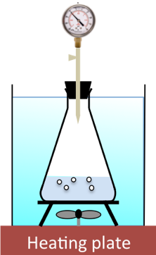
Real-time monitoring involves measuring a physical property of the system while the reaction is in progress. For example, a reaction that produces a gas can be monitored by measuring the volume of gas produced at different times with a syringe, or by noting the pressure of the gas at various time intervals with a pressure gauge (A). Another way to observe the progress of reaction in real-time is to record the change in mass of a reaction mixture over time (B).

The reaction between hydrochloric acid and calcium carbonate to give carbon dioxide is an example that can be monitored by either method A or B.

$2H_3O^+(aq)+CaCO_3(s)\rightarrow Ca^{2+}(aq)+CO_2(g)+3H_2O(l)$

Colorimetry, an analytical method to determine the concentration of dissolved coloured compounds, is also commonly used to observe the progress of a reaction (C). It begins with radiating the reaction mixture with a specific wavelength of light, which is selected by passing a continuum light source through a monochromatic filter. The monochromatic light is partly absorbed by the coloured compound before it exits the mixture. A detector then captures the exiting light and conveys the data to a computer for analysis. Since the amount of monochromatic light absorbed by the coloured species is proportional to the concentration of the species, the progress of the reaction can be monitored in real-time. The reaction between iodide and hypochlorite to form hypoiodite, which absorbs near 400 nm, is an example of a reaction that can be monitored using colorimetry:

$ClO^-(aq)+I^-(aq)\rightarrow IO^-(aq)+Cl^-(aq)$

Quenching methods, on the other hand, involve extracting a sample of the reaction mixture called an aliquot, quenching or stopping the reaction in the aliquot, and analysing the quenched mixture using other analytical techniques like titration (D), spectroscopy or chromatography. Some of the ways to quench a reaction mixture include:

1. Diluting a reaction mixture with water, e.g. for the decomposition of oxalic acid in concentration sulphuric acid.
2. Cooling a reaction suddenly, e.g. by spraying an aqueous reaction mixture with cold isopentane.
3. Adding a reagent that combines with one of the reactants to stop the reaction, e.g. adding acid to quench the hydrolysis of ethyl acetate in a basic solution.
4. Inactivating or removing a catalyst in a reaction mixture, e.g. adding a base in the acid-catalysed iodination of acetone to remove the catalyst:

$(CH_3)_2CO(l)+I_2(aq)\; \: \begin{matrix} H^+\\\rightarrow \end{matrix}\: CH_3COCH_2I(l)+HI(aq)$

Aliquots of the reaction mixture are extracted over several time intervals and added to excess aqueous sodium hydrogen carbonate to neutralise the acid. The concentration of the remaining iodine is then determined by titration with sodium thiosulphate.

Next article: Analysing rate data

Previous article: Half-life

Content page of intermediate chemical kinetics

Content page of intermediate chemistry

Main content page

November 4, 2019December 30, 2025

Analysing rate data (chemical kinetics)

The aim of analysing rate data from an experiment is to determine the reaction order with respect to different reactants, the rate constant, and hence the rate law.

Although various approaches can be employed to achieve this, depending on the type of reaction being investigated, most experimental procedures are structured in a way that narrows the approaches down to one or two.

The commonly used methods for analysing rate data are:

1. the half-life method
2. the differential method
3. the integral method
4. the initial rate method; and
5. the isolation method

Some experiments may require a combination of these methods to derive the rate equation. We shall look at them individually and see how they can be used.

Next article: Half-life method

Previous article: Monitoring the progress of a reaction

Content page of intermediate chemical kinetics

Content page of intermediate chemistry

Main content page

November 4, 2019December 12, 2024

Half-life method

The half-life method for analysing rate data is useful when the rate law involves a single reactant, i.e.

$rate=k[A]^i\; \; \; \; \; \; \; \; 22$

To determine the values of k and i, we let the reaction proceed, measure the appropriate physical property and plot the data in a concentration versus time graph.

If the curve is a straight line (see graph above), the gradient or the change in concentration versus the change in time (i.e. rate of reaction) is a constant. This implies that i = 0 in eq22, i.e. a zero order reaction. We can further confirm this by finding the first three successive half-lives from the graph (there is no need to consider the subsequent half-lives) and substitute them, along with the initial concentration of the reactant, in eq20 from the article on half-life: $t_{\frac{1}{2}}=\frac{[A]_0}{2k}$ . The three substitutions should give three different values of k that should be close to one another. The average of these values of k is then taken to give the rate equation: rate = k_ave.

If the curve is concave (see diagram above), it represents a higher order reaction. Similarly, the first three successive half-lives is determined from the graph. If the values are relatively constant, the graph corresponds to a first order reaction, with i = 1. The value of the rate constant is then found using eq19 from the article on half-life: $t_{\frac{1}{2}}=\frac{ln2}{k}$ , resulting in the rate equation: rate = k[A].

If the half-lives are very different from one another, they could be those of a second order reaction, i = 2. We can verify this by substituting the three half-life values, along with the initial concentration of the reactant, in eq21 from the article on half-life: $t_{\frac{1}{2}}=\frac{1}{k[A]_0}$ , which should give three different values of k that may be close to one another. The average value of the rate constant can be found and hence, the rate equation: rate = k_ave[A]².

Next article: Differential method

Previous article: Analysing rate data

Content page of intermediate chemical kinetics

Content page of intermediate chemistry

Main content page

November 4, 2019September 25, 2024

Differential method (rate laws)

The differential method of determining the rate of a reaction makes use of the differential form of a rate law.

Just like the half-life method, the differential method is useful for reactions involving a single reactant, e.g.

$N_2O_5(g)\rightleftharpoons 2NO_2(g)+\frac{1}{2}O_2(g)$

where we can write the rate equation as

$-\frac{d[N_2O_5]}{dt}=k[N_2O_5]^i\; \; \; \; \; \; \; \; 23$

Taking the natural logarithm on both sides of eq23, we have

$ln\left [ -\frac{d[N_2O_5]}{dt} \right ]=iln[N_2O_5]+lnk\; \; \; \; \; \; \; \; 24$

To find the rate constant, k, and the order, i:

1. Run the experiment in a rigid vessel and record the concentrations of N₂O₅using spectroscopic methods at various times.
2. Plot a graph of [N₂O₅] versus time.
3. Find the gradients to the curve at selected concentrations; that is, find $\frac{d[N_2O_5]}{dt}$ at various [N₂O₅].
4. With reference to eq24, plot a graph of $ln\left [- \frac{d[N_2O_5]}{dt} \right ]$ versus ln[N₂O₅] using the values determined in step 3.

The gradient and the vertical intercept of the line in the second graph give the values of i and lnk respectively. The differential method is commonly used together with the initial rate method and the isolation method in determining the unknowns of a rate equation with multiple reactants.

Next article: Integral method

Previous article: Half-life method

Content page of intermediate chemical kinetics

Content page of intermediate chemistry

Main content page

November 4, 2019November 16, 2025

Rate laws – integral form

An integral rate law mathematically expresses the rate of a reaction in terms of the initial concentration and the measured concentration of one or more reactants over a particular time.

Such a rate law can be derived from its differential form via simple calculus. Consider the decomposition of hydrogen peroxide to oxygen:

$H_2O_2(aq)\rightleftharpoons H_2O(l)+\frac{1}{2}O_2(g)$

The rate law is experimentally determined to be first order: rate = k[H₂O₂]. If we are monitoring the progress of the reaction by measuring the change in concentration of the peroxide, the differential form of the rate law is:

$-\frac{d[H_2O_2]}{dt}=k[H_2O_2]\; \; \; \; \; \; \; \; 12$

Rearranging and integrating eq12 gives:

$\int_{[H_2O_2]_0}^{[H_2O_2]}\frac{1}{[H_2O_2]}d[H_2O_2]=-k\int_{0}^{t}dt$

where [H₂O₂]₀ is the concentration of the peroxide at t = 0, i.e. its initial concentration.

We then get:

$ln\frac{[H_2O_2]}{[H_2O_2]_0}=-kt\; \; \; or\; \; \; ln[H_2O_2]=-kt+ln[H_2O_2]_0\; \; \; \; \; \; \; \; 13$

Eq13 is the integral form of the first order rate law for the decomposition of hydrogen peroxide. The general equation for a species, A, that participates in a first order reaction of vA → B is:

$ln\frac{[A]}{[A]_0}=-vkt\; \; \; or\; \; \; ln[A]=-vkt+ln[A]_0\; \; \; \; \; \; \; \; 14$

For a zero order reaction, e.g. the decomposition of excess N₂O on hot platinum, $N_2O\rightarrow N_2+\frac{1}{2}O_2$ , the rate equation is $-\frac{d[N_2O]}{dt}=k$ . Integrating both sides of this differential rate equation yields:

$[N_2O]=-kt+[N_2O]_0\; \; \; \; \; \; \; \; 15$

In general, a species, A, that participates in a zero order reaction of vA → B has the equation:

$[A]=-vkt+[A]_0\; \; \; \; \; \; \; \; 16$

For a second order reaction, e.g. NO₂ + CO → NO + CO₂ , the rate equation is:

$-\frac{d[NO_2]}{dt}=k[NO_2]^2$

and its integral form is:

$\frac{1}{[NO_2]}=kt+\frac{1}{[NO_2]_0}\; \; \; \; \; \; \; \; 17$

Once again, the generic second order rate equation that involves only one species, A, in a reaction, vA → B, is:

$\frac{1}{[A]}=vkt+\frac{1}{[A]_0}\; \; \; \; \; \; \; \; 18$

Finally, the diagram below shows the combined concentration-time plot of eq14, eq16 and eq18 for a chemical species A.

Next article: Half-life

Previous article: Units of a rate constant

Content page of intermediate chemical kinetics

Content page of intermediate chemistry

Main content page

November 4, 2019October 27, 2024

Integral method (chemical kinetics)

The integral method of determining the rate of a reaction makes use of the integral form of a rate law.

Just like the half-life method and the differential method, the integral method is useful for reactions involving a single reactant, e.g.

$N_2O_5(g)\rightleftharpoons 2NO_2(g)+\frac{1}{2}O_2(g)$

If the order of the reaction is known, we can determine the value of the rate constant by plotting the appropriate integral rate equations below using experiment data and finding the vertical intercept of the respective linear functions.

Order	Rate law	Integral rate equation
0	$rate=k$	$[A]=-kt+[A]_0$
1	$rate=k[A]$	$ln[A]=-kt+[A]_0$
2	$rate=k[A]^2$	$\frac{1}{[A]}=kt+\frac{1}{[A]_0}$

If the order of the reaction is not known, the integral rate equation that gives a straight line with the experiment data is the one that describes the order of the reaction. The integral method can also be used together with the initial rate method and the isolation method in determining the unknowns of a rate equation with multiple reactants.

Next article: Initial rate method

Previous article: Differential method

Content page of intermediate chemical kinetics

Content page of intermediate chemistry

Main content page

November 4, 2019September 25, 2024

Initial rate method (chemical kinetics)

The rate of a reaction decreases with time because the concentrations of reactants decrease as a reaction progresses. This poses a problem when we want to compare reactions under different conditions, e.g. to compare the reaction rates for different concentrations of HCl on CaCO₃.

The diagram above shows the pressure of CO₂ liberated over time for the reaction of CaCO₃ with HCl at three different concentrations: A, B and C. Instead of arbitrarily choosing points on each curve to determine the gradients and hence the respective reaction rates (upper left graph), a basis of comparison must be established before finding the gradients. The initial rate of reaction (i.e. the gradient at t ≈ 0, just after the start of the reaction) is eventually chosen as the reference point (upper right graph), because the concentrations of HCl are approximately the same as that before the start of the respective reactions, especially for slow reactions. It is also chosen partly to minimise the effects of temperature (from exothermic or endothermic reactions) on the system when the reaction progresses. Furthermore, the initial rate of reaction method is useful for studying the forward reaction rate of a reversible reaction where the reverse reaction is negligible at the start. The initial rate method can be used to determine rate equations involving either a single or multiple reactants.

To illustrate the method, consider a constant volume reaction with the rate law:

$R=k[A]^i\; \; \; \; \; \; \; \; 25$

The experiment is carried out with four different initial concentrations of the reactant, A, with the data plotted in a concentration versus time graph (see diagram below).

Since,

$R=\frac{change\, in\, concentration\, of \, reactants\, or\, products}{\, change\, in\, time}$

the four gradients of the curves a, b, c and d are the rates of the respective reactions at t = 0, i.e. the initial rates. Taking the natural logarithm of both sides of eq25, we have

$lnR=lnk+iln[A]\; \; or\; \; lnR_0=lnk+iln[A]_0\; \; \; \; \; \; \; \; 26$

where R₀ and [A]₀ are the initial rate of reaction and initial concentration of A respectively. If we plot the natural logarithm of the initial reaction rates of the four curves against the natural logarithm of the respective initial concentrations of A, we get a straight line with gradient i and vertical intercept lnk. Therefore, the rate constant and the order of eq25, and hence the entire rate law, can be found.

Next article: rate laws – integral form

Previous article: Order of a reaction

Next article: Units of a rate constant

Previous article: Rate laws – differential form

Next article: Monitoring the progress of a reaction

Previous article: Rate laws – integral form

Next article: Analysing rate data

Previous article: Half-life

Next article: Half-life method

Previous article: Monitoring the progress of a reaction

Next article: Differential method

Previous article: Analysing rate data

Next article: Integral method

Previous article: Half-life method

Next article: Half-life

Previous article: Units of a rate constant

Next article: Initial rate method

Previous article: Differential method

Next article: Why is initial rate proportional to 1/t?

Previous article: Integral method