Colligative properties are physical properties of solutions that depend solely on the number of solute particles present, not on their chemical identity. The term “colligative” comes from the Latin word colligatus, meaning “bound together”, reflecting the idea that these properties arise from the collective presence of solute particles, regardless of their type, size or chemical nature.
The classical treatment of colligative properties rests on two key assumptions:
-
- The solute is non-volatile — only the solvent contributes to the vapour phase, so any change in vapour pressure (and related properties) comes solely from the dilution of the solvent.
- The solution behaves ideally — solute and solvent molecules interact only through simple physical mixing, with no strong intermolecular forces altering the behaviour of the components. Dilute non-ideal solutions behave nearly ideally at low solute concentrations and also exhibit colligative properties.
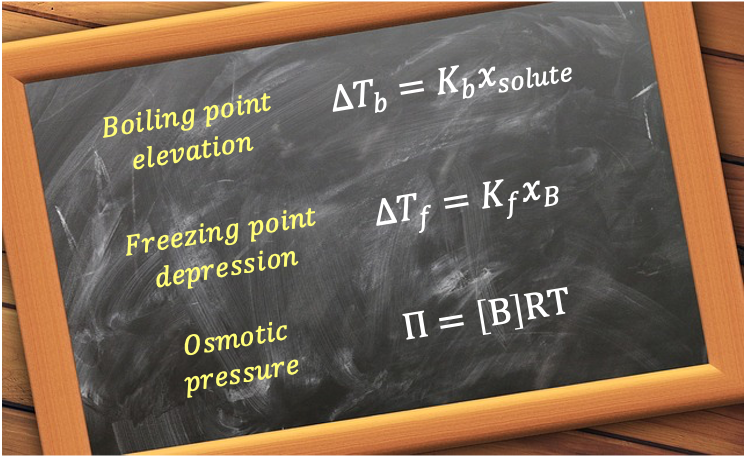
The four principal colligative properties are vapour pressure lowering, boiling point elevation, freezing point depression and osmotic pressure. As vapour pressure lowering has been discussed in the article on Raoult’s law, we will elaborate on the remaining properties.
Boiling point elevation
The normal boiling point of a pure liquid or solution is the temperature at which its vapour pressure equals 1 atm. According to Raoult’s law, the addition of a non-volatile solute to a pure liquid lowers the vapour pressure of the solvent. As a result, a higher temperature is required for the solution’s vapour pressure to reach 1 atm. Therefore, the normal boiling point of the solution is elevated relative to that of the pure solvent.
To explain this mathematically, consider a volatile solvent and a nonvolatile solute in a solution at equilibrium with the gaseous solvent at a constant pressure. Raoult’s Law states that at any given temperature, the vapour pressure of the solvent in the solution is related to the vapour pressure of the pure solvent at that same temperature. Using eq178 at the solution’s boiling point , we have
where is the external pressure and
denotes the vapour pressure of the solution at
.
Since the pure solvent boils at , we have
, which when combined with eq189 gives
As the Clausius-Clapeyron equation describes how the vapour pressure of a substance changes with temperature, we can express eq169 as:
Substituting eq190 into eq191 yields
For dilute solutions, . So, the Taylor expansion of
becomes
, and
where .
Assuming that for a dilute solution and
is independent of temperature, eq192 becomes
where .

Question
If , why isn’t
?
Answer
Even if , there is still some small elevation in boiling point when
increases. Another way to proceed from eq192 is to rearrange it to:
Let and
Using the Taylor expansion of , we have
for small
, and eq193a rearranges to eq193.
Freezing point depression
Freezing is the process by which a liquid transforms into a solid with an ordered, crystalline structure. When a non-volatile solute is added to the solvent, it effectively dilutes the solvent and increases the entropy of the solution. The reduction in the concentration of solvent molecules, along with the enhanced molecular randomness, opposes the tendency of the solution to freeze (freezing lowers the entropy of the system). As a result, a lower temperature is required for freezing to occur.
Consider a pure solid (A) at equilibrium with a solution containing the dilute solute (B). Since the chemical potentials of A in the two phases are equal at equilibrium, eq181 becomes
Dividing eq194 by and differentiating it with respect to
at constant
gives
Question
Show that .
Answer
Using the quotient rule,
From eq173, . So,
Combining eq143 and eq149a, we have , and
Therefore, eq195 becomes , or equivalently,
where .
Assuming is independent of temperature and integrating both sides of eq196 with respect to
yields,
The limits of integration represent a transition from the normal freezing temperature of pure solvent A (where
) to the depressed freezing point of the solution
(where
). Therefore,
For dilute solutions, . So, the Taylor expansion of
and
Assuming that for a dilute solution,
where is the freezing point depression and
.
Osmotic pressure
Osmosis is the tendency of pure solvent molecules A to diffuse across a semipermeable membrane into a solution of A and B. Consider two equal chambers separated by a rigid, thermally conducting, semipermeable membrane that allows only molecules of solvent A to pass through, but not solute B (see diagram below). In the left chamber is pure solvent A. In the right chamber, we have a solution of B in A. Initially, the heights of the liquids in the two capillary tubes connected to the chambers are equal, so the pressures in both chambers are the same (). Furthermore, the membrane conducts heat and thermal equilibrium is maintained.
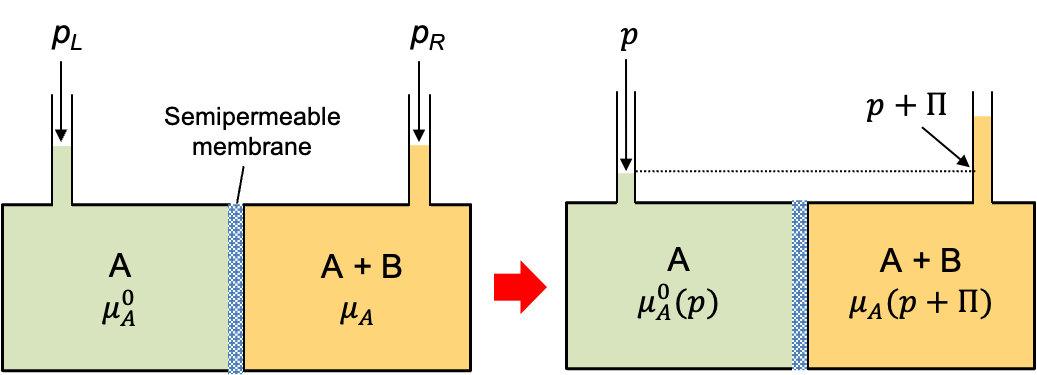
The chemical potential of pure solvent A in the left chamber is denoted by . In the right chamber, the presence of solute B lowers the chemical potential of A, so
. The resulting chemical potential difference indicates that the system, being out of equilibrium, will spontaneously evolve to minimise its Gibbs energy. This is achieved by solvent A flowing from the pure solvent side through the semipermeable membrane into the solution, thereby diluting the solute and raising the chemical potential of A in the right chamber.
As solvent flows into the right chamber, the liquid level in its capillary tube rises, increasing the hydrostatic pressure in that chamber. This pressure buildup continues until the chemical potentials of the solvent in both chambers are equal. At that point, equilibrium is restored and the additional pressure generated in the right chamber is called the osmotic pressure. The magnitude of this pressure reflects the extent of osmosis that has occurred in the system and enables quantification of that extent.
When equilibrium is restored, . Using eq181, we have
Integrating eq173 at constant , we have
or
Substituting eq198 into eq199 yields
For dilute solutions, . So, the Taylor expansion of
and
Substituting and
for dilute solutions, and
in eq200 gives
Eq201 is called the van’t Hoff law, which describes the osmotic pressure of an ideal-dilute solution. For non-ideal solutions, the osmotic pressure can be approximated using a power series expansion analogous to the virial expansion for real gases:
where ,
are osmotic virial coefficients that capture non-ideal interactions.