The three-electrode cell is used to measure the activation overpotential of a cell at various levels of current. Consider the following experiment setup:
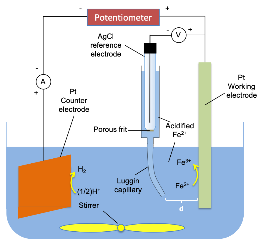
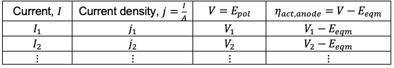
The opening end of the Luggin capillary is brought very close to the working electrode (d≈0) and the potential of the working electrode Eeqm is measured with the potentiometer and counter electrode removed from the circuit. The two are then reconnected to the circuit and the externally applied potential is turned on to a magnitude greater than 0.57 V (e.g. 0.8V), resulting in Fe2+ being oxidised to Fe3+ at the anode and H+ reduced to H2 at the cathode. The potential of the working electrode Epol is again recorded. Assuming that the electrolyte is well-stirred, the difference between Epol and Eeqm is the activation overpotential of the anode with respect to the current flowing at 0.8 V. By increasing the applied potential, we can tabulate the increasing levels of current, I, flowing in the circuit (see table below) and consequently record the corresponding overpotentials ηact,anode using eq61.

If the overpotential at the anode is greater than +100 mV, the second exponential in the Butler-Volmer equation tends to zero, giving:
This means that the net current density at the anode mainly comprises of anodic current density. Taking natural logarithm on both side of eq69,
Eq70 is known as the Tafel equation, named after the Swiss chemist, Julius Tafel. The plot of ln(I/A) against η is called a Tafel plot and it allows us to find the value of the transfer coefficient from the gradient of the line and the exchange current density j0 from the intercept. Such an experiment that monitors current at various potentials is called voltammetry.
The three-electrode cell can also be modified slightly to measure the total overpotential of a cell, . Consider the following experiment with metallic copper for both the anode and cathode, and AgCl electrode as the reference electrode.
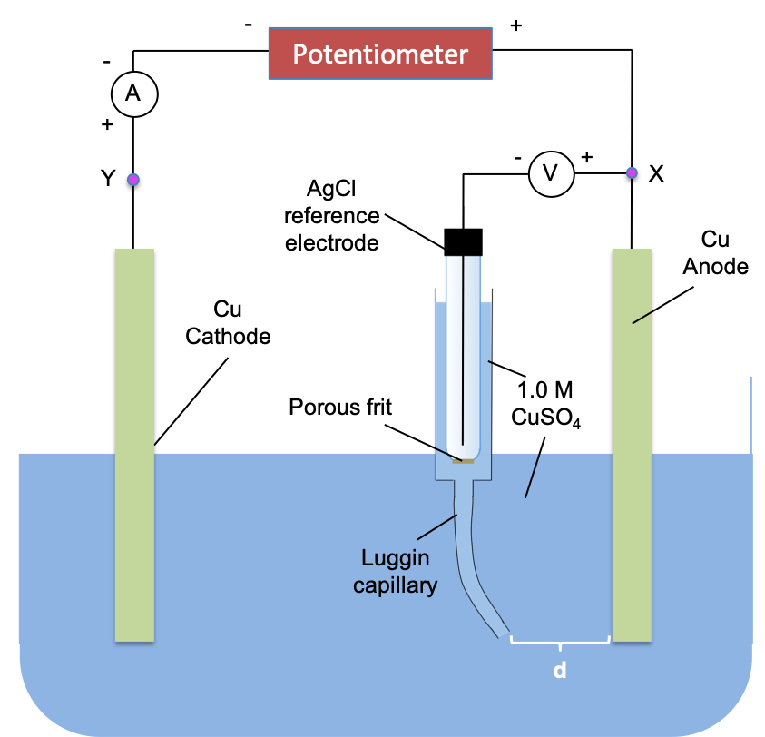
With the potentiometer set to 0 V,
-
- Measure potential of the left electrode EL, eqm by connecting the reference electrode to junction X.
- Measure potential of the right electrode ER, eqm by connecting the reference electrode to junction Y.
We’d expect EL, eqm = ER, eqm. Next, turn the potentiometer to 1.0 V and
-
- Measure potential of the left electrode (anode) Ean, pol by connecting the reference electrode to junction X.
- Measure potential of the right electrode (cathode) Ecat, pol by connecting the reference electrode to junction Y.
We’d expect Ean, pol > EL, eqm and Ecat, pol < ER, eqm.
We can also measure IR drop (in mV/cm) for the above setup by setting the external applied voltage at 1.0 V and measuring the anode potential at different Luggin capillary distances, d.