Pressure-composition diagrams are graphical representations that illustrate the relationship between the vapour pressures of components in a liquid mixture and their compositions at a constant temperature. These diagrams are essential tools in physical chemistry and chemical engineering, particularly for understanding phase equilibria in binary mixtures.
Ideal solution
Consider two liquids A and B (e.g. benzene and toluene) forming an ideal solution in a closed container (e.g. a container with a movable piston) at a constant temperature above the freezing points of both species. The partial pressures of the components follow Raoult’s law:
where
is the partial vapour pressure of component
is the vapour pressure of pure
is the mole fraction of
in the solution
The total vapour pressure of the ideal solution is:
According to Dalton’s law, the mole fractions and
of the components in the gas are
Substituting eq189 and eq190 in eq191 results in
Substituting in eq189 into
in eq191 gives
Substituting eq193 in of eq192 and rearranging yields
Eq190 and eq194 are plotted in a graph of against
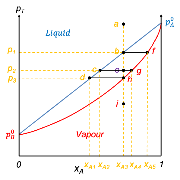
to produce the pressure-composition diagram of the ideal solution (see diagram above). Eq190, also known as the liquid composition curve, describes a straight line (blue) along which the liquid begins to vaporise. In other words, the high pressure region above this line corresponds to the liquid phase of the solution. In contrast, eq194 defines the curve (red) along which the last drop of the liquid vaporises. The region below this curve, also called the vapour composition curve, represents the vapour phase. The area between eq190 and eq194 marks the two-phase region where liquid and vapour coexist in equilibrium.

Question
What is ? Isn’t the graph plotted against
and
?
Answer
is the overall mole fraction of A in the system, including both the liquid and vapour phases. It ranges from 0 to 1 and is given by:
When we plot eq190 and eq194, we are plotting them against and
respectively. These values also lie between 0 and 1. However, neither
or
can define all the points in the liquid, vapour and two-phase regions. Therefore, after plotting the two equations, we replace the horizontal axis with
, which allows a single, continuous representation of the system’s behaviour across all regions. When interpreting the horizontal axis at a point along eq190, we consider the case where
, which gives
Similarly, at a point along eq194, we assume , resulting in
.
Consider the process of isothermally lowering the pressure from point a to i (see diagram above), which can be achieved by drawing out the piston. At point a, the pressure is above eq190 at . Under these conditions, the system is entirely in the liquid phase. As the pressure is reduced to point b, the system reaches the liquid composition curve. Here, the first infinitesimal amount of vapour forms, and the system enters a two-phase equilibrium. At this point, the liquid composition is still equal to the overall composition (
), but the vapour phase has a different composition corresponding to point f (
). A tie-line bf on the diagram connects these two phase compositions, indicating that both phases coexist in equilibrium.
Continuing to lower the pressure brings the system to point e, which lies between the two curves. This is the two-phase region, where both liquid and vapour coexist in significant amounts. The overall composition remains fixed at , but the compositions of the individual phases are
(point c) and
(point g) for the liquid phase and vapour phase respectively.
When the system reaches point h on the vapour composition curve, the last drop of liquid evaporates. At this point, the liquid phase composition is (), and the vapour phase composition matches the overall composition (
). Finally, as the pressure is reduced even further to point i, the system moves below the vapour composition curve, where it exists as a single-phase vapour. No liquid remains and the composition remains constant at
. The line abehi is called an isopleth.
Question
Why is the overall composition of the system fixed at when the pressure is reduced?
Answer
is the overall mole fraction of A in the system, including both the liquid and vapour phases. In the closed container, the total number of moles of component A and B remains constant — just distributed differently between liquid and vapour when pressure is reduced.
Interestingly, even though the compositions of the phases are fixed at a given pressure (e.g. and
at
), the overall mole fraction of A can vary continuously between them, depending on the relative amounts of each phase. To understand this, let
be the number of moles of A in the liquid phase
be the number of moles of A in the vapour phase
be the total number of moles of A and B in the liquid phase
be the total number of moles of A and B in the vapour phase
be the total number of moles of A and B in the closed container
Clearly,
Substituting eq195 and eq196 into eq197 and rearranging gives
Since , the range of
is
, which corresponds to the domain of a tie-line at a particular pressure and temperature. Multiplying both sides of eq198 by
and rearranging yields
Substituting into eq199 and rearranging results in the lever rule:
Here, represents the length from the left end of a tie-line to the intersection of the tie-line and with the isopleth, while
represents the length from that intersection to the right end of the tie-line. Eq200 allows us to determine the relative amounts of the two phases in equilibrium by measuring these two lengths. This principle has important applications in material science and chemical engineering — for instance, in predicting phase amounts, which is critical for the design of distillation columns.
Non-ideal solution
Pressure-composition diagrams for non-ideal binary solutions typically exhibit two characteristic shapes, depending on the degree and nature of deviation from Raoult’s law. When the deviation is small, the liquid composition curve is monotonic, with no stationary points. In such cases, the diagram features two smooth curves that intersect only at and
(see diagram below). A typical example is the carbon tetrachloride-toluene system, where carbon tetrachloride is the more volatile component.
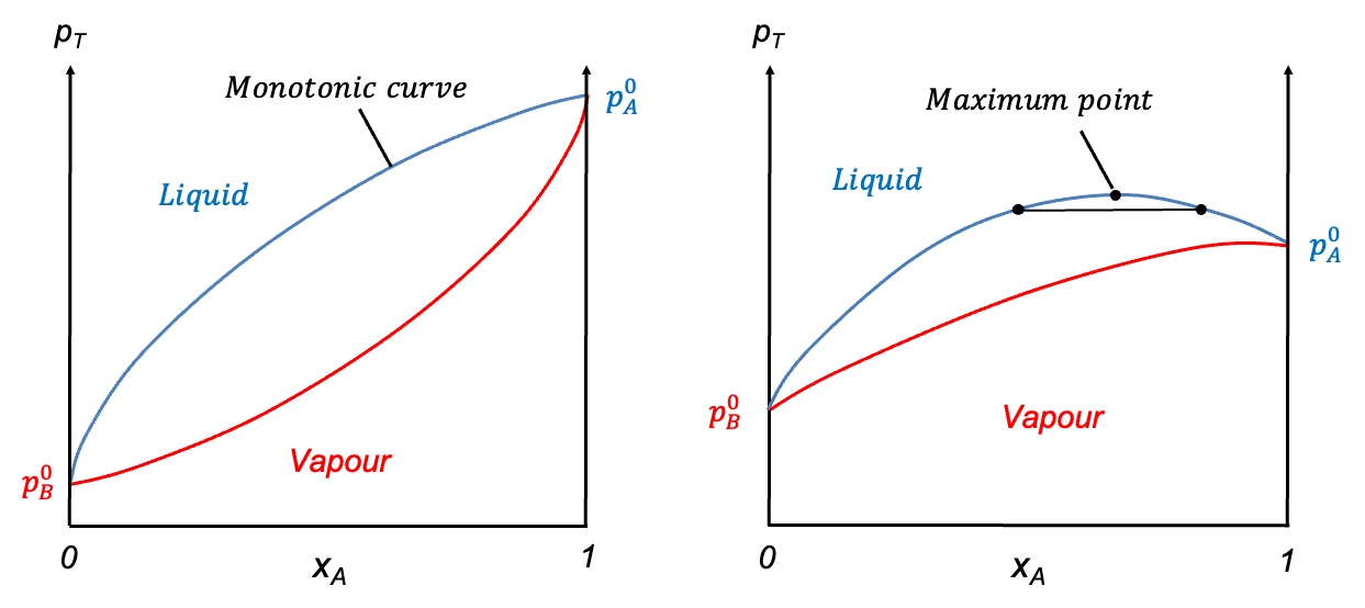
In contrast, when the deviation from Raoult’s law is significant, the liquid composition curve may develop a stationary point. The nature of this point is governed by the intermolecular interactions between components A and B. A maximum point occurs when A-B interactions are weaker than A-A and B-B interactions, while a minimum point arises when A-B interactions are stronger than A-A and B-B interactions.
Now consider a liquid composition curve with a maximum point. Suppose the corresponding vapour composition curve intersects the liquid composition curve only at and
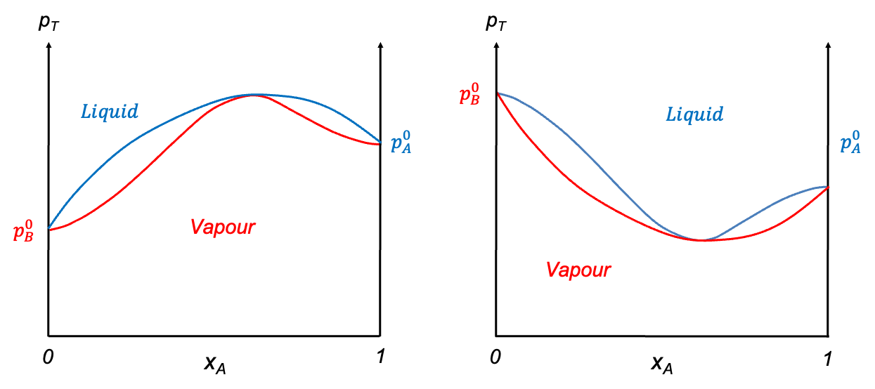
. In this case, a tie-line drawn just below the maximum point would connect two points on the liquid composition curve (see diagram above), implying two coexisting liquid phases at different compositions — a physical impossibility for a binary system in vapour–liquid equilibrium. This contradiction indicates that the vapour composition curve must also touch the liquid composition curve at the maximum point, as shown in the diagram below. A solution that behaves this way is called an azeotrope. The ethanol–water system is an example of an azeotrope with a maximum point, while the HCl–water system forms an azeotrope with a minimum point. These diagrams are typically constructed using empirical data.
Distillation
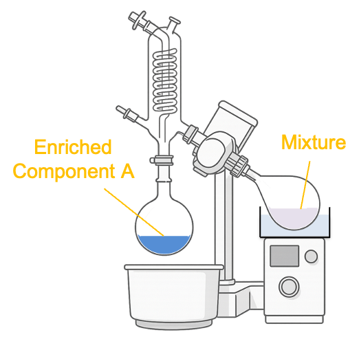
A rotary evaporator (see diagram below) separates the components of a binary mixture by reducing the pressure above the mixture with a vacuum pump. Pressure-composition diagrams can help predict the operating pressure required for distilling the more volatile component when using a rotary evaporator.
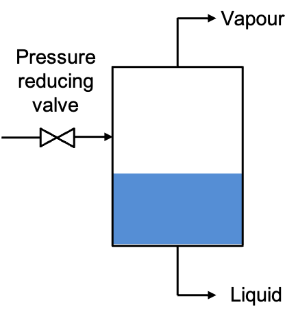
Pressure-composition diagrams are also used in flash distillation, which involves the partial vaporisation of a liquid mixture to separate its components based on differences in volatility. In a flash distillation process, a pre-heated liquid mixture is introduced into a flash drum or separator operating at a reduced pressure (see diagram below). Upon entry, a portion of the liquid “flashes” into vapour due to the sudden pressure drop. This generates two phases in equilibrium: a vapour phase enriched in the more volatile component, and a liquid phase enriched in the less volatile one. These two phases are then physically separated, with the vapour removed at the top and the liquid removed at the bottom. The phases can undergo further distillation, depending on the desired separation efficiency and purity of the components.
Pressure-composition diagrams are crucial in this context because they show how the equilibrium compositions of the vapour and liquid phases vary with pressure at a fixed temperature. These diagrams help determine the operating conditions (such as temperature and pressure) at which the desired separation can occur, as well as predict the relative amounts of vapour and liquid formed.
Flash distillation is widely used in the chemical and petroleum industries — for example, in crude oil refining — where it serves as a rapid, energy-efficient method for achieving partial separation of multi-component mixtures without the complexity of a full distillation column.