Temperature-composition diagrams are graphical representations that show the relationship between the boiling point (temperature) of a liquid mixture and the composition of the mixture at a constant pressure.
Ideal solution
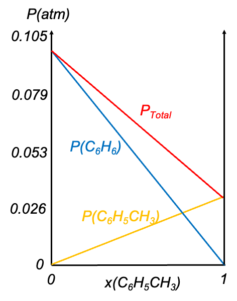
Consider two liquids A and B (e.g. benzene and toluene) forming an ideal solution in a closed container at a constant pressure  . The partial pressures of the components follow Raoult’s law:
\;\;\;\;\;\;\;\;p_B=x_{B,l}p_B^0(T))
where
 is the partial vapour pressure of component
) is the vapour pressure of pure as a function of
is the vapour pressure of pure as a function of 
 is the mole fraction of in the solution
The total vapour pressure of the ideal solution is equal to the fixed pressure: +(1-x_{A,l})p_B^0(T)) , which rearranges to
, which rearranges to
}{p_A^0(T)-p_B^0(T)}\;\;\;\;\;\;\;\;201)
Using known values of at different , eq201 is used to plot the liquid composition curve for a graph of against  (see diagram below). Substituting eq201 into
 }{p_T}) yields
yields
}{p_A^0(T)-p_B^0(T)}\frac{p_A^0(T)}{p_T}\;\;\;\;\;\;\;\;202)
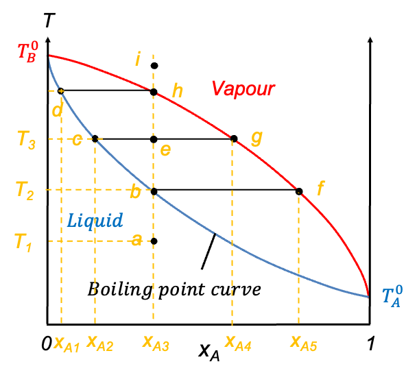
Eq202 describes the vapour composition curve. Unlike the pressure-composition diagram of an ideal solution, the vapour composition curve lies above the liquid composition curve (also known as the boiling point curve). The vapour phase corresponds to the region above the vapour composition curve, while the liquid phase lies below the liquid composition curve. Furthermore, neither curve is linear.

Question
Why is the liquid composition curve also called the boiling point curve?
Answer
At a fixed pressure  , boiling in a temperature–composition diagram refers to the phase change from liquid to vapour that occurs when the mixture’s vapour pressure equals or exceeds . The liquid composition curve defines the boundary at which this phase change begins.
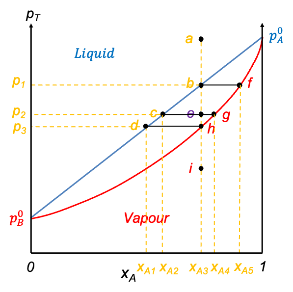
Similar to pressure-composition diagrams, the horizontal axis, after plotting the two curves, is relabelled as  , representing the overall mole fraction of A in the system, including both the liquid and vapour phases. Consider the process of isobarically increasing the temperature from point a to i (see diagram above). At point a, the system is entirely in the liquid phase. As the temperature is increased to point b, the system reaches the liquid composition curve. Here, the first infinitesimal amount of vapour forms, and the system enters a two-phase equilibrium. At this point, the liquid composition is still equal to the overall composition (
 ), but the vapour phase has a different composition corresponding to point f (
 ). A tie-line bf on the diagram connects these two phase compositions, indicating that both phases coexist in equilibrium. The lever rule, as discussed in the article on pressure-composition diagrams, can likewise be used to determine the relative equilibrium amounts of the two phases present at any stage of heating, provided the temperature and overall composition fall between the liquid and vapour lines.
Continuing to increase the temperature brings the system to point e, which lies between the two curves. This is the two-phase region, where both liquid and vapour coexist in significant amounts. The overall composition remains fixed at  , but the compositions of the individual phases are
  (point c) and
  (point g) for the liquid phase and vapour phase respectively.
Question
Why is the overall composition of the system fixed at when temperature is increased?
Answer
is the overall mole fraction of A in the system, including both the liquid and vapour phases. In the closed container, the total number of moles of component A and B remains constant — just distributed differently between liquid and vapour as temperature increases.
When the system reaches point h on the vapour composition curve, the last drop of liquid evaporates. At this point, the liquid phase composition is ( ), and the vapour phase composition matches the overall composition (
 ). Finally, as the temperature is increased even further to point i, the system exists as a single-phase vapour. No liquid remains and the composition remains constant at . The line abehi is called an isopleth.
Question
Why does the mixture boil at a single temperature, instead of the more volatile component boiling off completely before the other begins to boil?
Answer
In a mixture, boiling occurs when the total vapour pressure — the sum of the partial vapour pressures of all volatile components — equals the external pressure. This means the mixture doesn’t boil when each component individually reaches its own boiling point, but rather when their combined vapour pressures are sufficient to match the external pressure. Both components vaporise simultaneously, but in proportions that depend on their relative volatilities. For example, although pure benzene boils at a lower temperature (80 °C at 1 atm) than pure toluene (111 °C at 1 atm), benzene’s vapour pressure in a mixture is reduced due to dilution by toluene, as described by Raoult’s Law. Benzene alone cannot reach the external pressure unless it is pure — and the same applies to toluene. Only together can their partial vapour pressures sum to equal the external pressure, allowing the mixture to boil.
Non-ideal solution
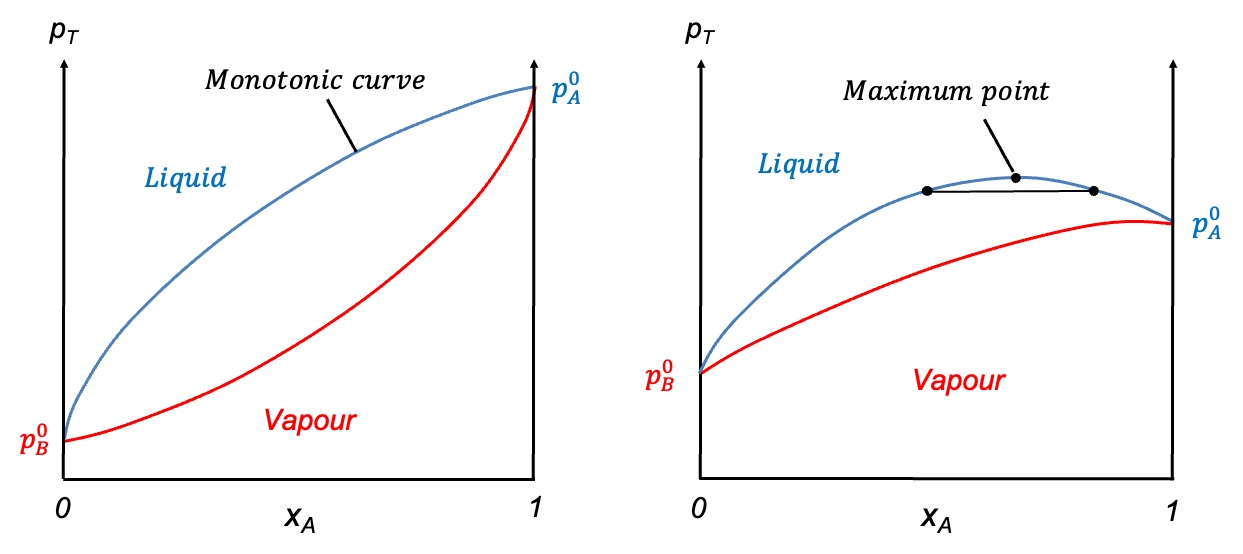
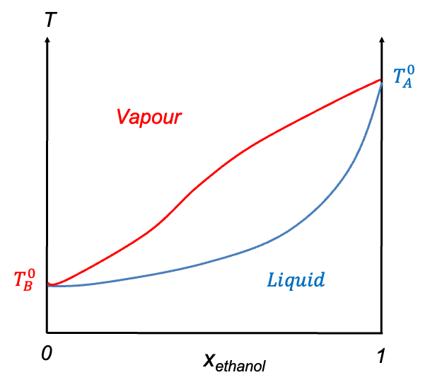
Temperature-composition diagrams for non-ideal binary solutions typically exhibit two characteristic shapes, depending on the degree and nature of deviation from Raoult’s law. When the deviation is small, the diagram features two smooth monotonic curves intersecting only at  and
and  (see diagram below). A typical example is the diethyl ether–ethanol system. Such a diagram has the same structure as that of an ideal solution, but differs in the curvature of the curves.
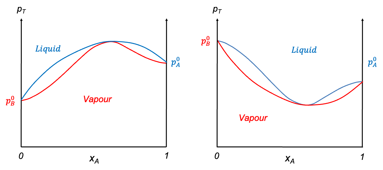
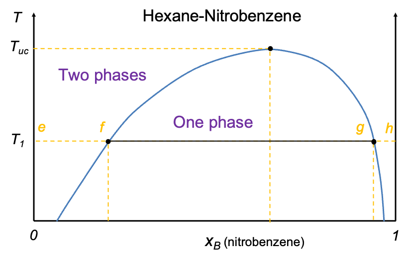
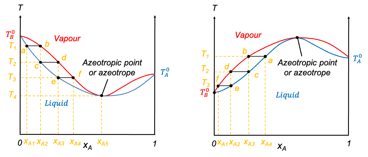
In contrast, when the deviation from Raoult’s law is significant, the curves may develop a stationary point. The nature of this point is governed by the intermolecular interactions between components A and B. When A-B interactions are weaker than A-A and B-B interactions, a minimum point may occur, as the mixture exhibits higher vapour pressures than predicted, resulting in lower boiling points. Conversely, if A-B interactions are stronger, a maximum point may form due to lower vapour pressures, which lead to higher boiling points than expected. Mixtures with such characteristics are called azeotropes. The ethanol–water system is an example of an azeotrope with a minimum point, while the HCl–water system has a maximum point (see diagram below). These diagrams are typically constructed using empirical data.
Question
Why must the two curves of an azeotrope intersect at the stationary point?
Answer
See this article for explanation.
Distillation
Temperature-composition diagrams are essential tools in understanding and designing simple and fractional distillation processes.
Consider the ethanol–water system (see above diagram). In simple distillation, the mixture ) is heated until it reaches its boiling point
is heated until it reaches its boiling point ) and begins to vaporise. At this stage, the vapour composition of ethanol is
and begins to vaporise. At this stage, the vapour composition of ethanol is  (point b), which is richer in ethanol. This vapour is then condensed and collected as the distillate, effectively separating it from the original mixture. Since this process involves just a single equilibrium between the liquid and vapour phases, it is typically considered a one-step separation. By using the diagram, one can estimate how effective the process will be for a single distillation step. However, simple distillation has its limitations. It provides only a partial enrichment of the more volatile component. For mixtures requiring higher purity, more advanced techniques like fractional distillation are necessary.
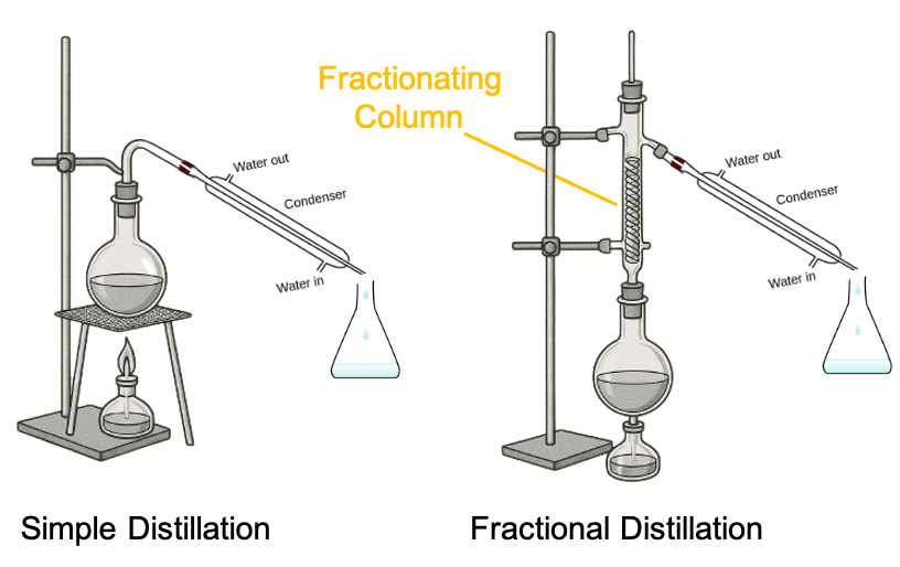
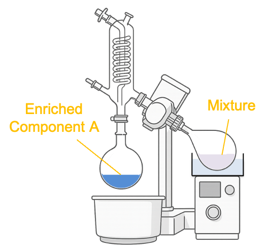
The fractional distillation apparatus used in the laboratory includes a fractionating column filled with glass beads, which provide a large surface area for repeated condensation and vaporisation cycles (see diagram above). Suppose the initial overall mole fraction of ethanol in the mixture is  (with reference to the minimum azeotrope diagram above). When the temperature reaches
  , the vapour in equilibrium with the liquid has an ethanol composition of , which is richer in ethanol due to its greater volatility. As this vapour rises through the fractionating column, it encounters a cooler region at temperature
  , where part of it condenses into a liquid with the same composition . The remaining uncondensed vapour becomes even more enriched in ethanol, now with composition . This ethanol-riched vapour continues to ascend, repeating the cycle: it partially condenses into liquid of composition , and leaves behind a vapour of even higher ethanol content,
  .
.
The condensation and vaporisation cycle continues as long as the column is tall enough to provide sufficient equilibrium stages. Eventually, the vapour composition reaches  , which corresponds to the azeotropic point — the minimum boiling point of the ethanol–water system. At this composition, the mixture behaves like a pure substance and boils at a constant temperature,
  . No further separation by distillation is possible beyond this point. Each individual equilibrium step in the fractional distillation process is referred to as a theoretical plate. For an ethanol-water mixture to reach azeotropic purity, typically 8 to 10 theoretical plates are needed. This can be achieved in the lab using a well-packed fractionating column of 50 to 70 cm in height.
At the top of the column, the azeotropic vapour is directed into the condenser, while the condensed liquid within the column flows back down towards the boiling flask, diluting the boiling mixture. The final composition of the distilled ethanol depends on this azeotropic limit, which is approximately 95.6% ethanol by mass at atmospheric pressure ( ).
).
Question
What happens if the starting mixture, containing a 0.92 mole fraction of ethanol, is heating to a temperature between  and ?
and ?
Answer
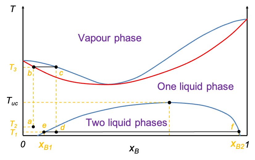
The final composition of the distillate contains 0.895 mole fraction of ethanol, while the residue will be richer in ethanol ( ).
).

Temperature-composition diagrams are essential tools in understanding and optimising fractional distillation, particularly in complex mixtures like petroleum. In an industrial fractional distillation column (see above diagram), crude oil is first heated in a furnace until it partially vaporises. The resulting vapour enters the base of the column (reboiler section) and rises through a series of trays or packing. Components with lower boiling points condense on trays higher up in the column (where temperatures are cooler), while components with higher boiling points condense on trays lower down (where it is hotter).
Although temperature–composition diagrams are typically illustrated for binary mixtures, the same principles can be conceptually applied to the multi-component mixture of crude oil. At different heights in the column, the mixture can be approximated as a “pseudo-binary” system, where one component (A) represents a heavier fraction and the other component (B) represents a lighter fraction. At a given temperature (i.e. at a particular tray), the vapour phase will be richer in the more volatile component B (lower boiling point), while the liquid phase will be richer in component A (higher boiling point). This vapour–liquid equilibrium process repeats over many stages, progressively enriching the vapour in more volatile components and enabling effective separation based on differences in volatility.