Advanced Chemistry

April 7, 2026April 8, 2026

Why lithium-ion batteries sometimes catch fire

Lithium-ion batteries power everything from smartphones and laptops to electric vehicles and energy storage systems. They are efficient, lightweight and rechargeable. However, under certain conditions, they can overheat, expand and even catch fire. Understanding why this happens comes down to how these batteries are built and what can go wrong inside them.

A lithium-ion battery consists of three key components: anode, cathode and the electrolyte (see diagram above). Separating the anode and cathode is a thin porous membrane called the separator, which plays the critical role of keeping the two electrodes apart while still allowing ions to pass through. As the battery charges and discharges, lithium ions shuttle back and forth between the electrodes, storing and releasing energy.

Under normal conditions, lithium-ion batteries are safe. Problems arise when internal or external factors disrupt their delicate balance, with the most serious outcome being thermal runaway — a chain reaction in which rising temperature accelerates further heat generation. The main trigger for a thermal runaway is an internal short circuit, which occurs when the anode and cathode come into direct contact. When this happens, charges no longer flow through the higher-resistance electrolyte, but instead travel via a very low-resistance path between the electrodes. This surge in internal current flow results in rapid heat generation that can lead to combustion.

So what causes the anode and cathode to come into direct contact? Physical damage, such as dropping, crushing or puncturing a battery can deform its internal structures. Manufacturing defects may leave contaminants, like metal particles or dust, inside the battery that can pierce the separator. Another cause is lithium plating, which can lead to dendrite growth.

Lithium plating occurs when lithium ions deposit as metallic lithium on the surface of the anode, Li⁺(aq) + e^– → Li(s), instead of moving into the anode’s internal structure (a process known as intercalation). Fast charging drives lithium ions rapidly towards the anode and can overload its surface. If the intercalation rate is slower than the incoming flux, the excess ions tend to accumulate and are reduced to metallic lithium on the anode surface. Low operating temperatures (< 273.15 K), which increase the viscosity of the electrolyte and decrease ionic mobility, can also promote lithium plating (the slower diffusion of ions into the graphite layers causes them to accumulate and plate onto the surface).

Initially, this plated lithium layer is often relatively uniform, so the anode and cathode remain physically separated by the separator, although the battery capacity may be affected. However, if the plated lithium grows unevenly over time, it can form needle-like structures called dendrites. These body-centred cubic structures can pierce the separator and reach the cathode, creating a direct, low-resistance path between the electrodes and leading to an internal short circuit.

Finally, gas buildup in a lithium-ion battery, caused by electrolyte decomposition over time, can also result in thermal runaway. This decomposition involves the battery’s electrolyte, which typically consists of the lithium salt LiPF₆ dissolved in an organic solvent such as ethylene carbonate or dimethyl carbonate. Under stress (e.g. overcharging or high temperature), LiPF₆ can decompose to PF₅ (LiPF₆ → LiF + PF₅), which then reacts with trace amounts of water to produce hydrogen fluoride gas (PF₅ + 4H₂O → H₃PO₄ + 5HF). The organic solvents can also oxidise or decompose, producing gases like CO, CO₂ or hydrocarbons, leading to battery swelling commonly observed as bulging laptop casings. The increased internal pressure may displace the electrodes, causing an internal short circuit, or even rupture the battery. This significantly increases the risk of explosion, especially if the gases are flammable.

To mitigate such risks, high-quality lithium-ion battery designs use a combination of materials, architecture and protective systems to prevent lithium plating, dendrite formation, gas buildup, and short circuits. For instance, high-quality graphite, silicon-graphite composites or lithium titanate anodes ensure even lithium intercalation, reducing the risk of plating. Additives are also included in the electrolyte to regulate lithium deposition and suppress dendrite growth. Furthermore, multi-layer microporous polymer separators can resist puncture by dendrites.

Additionally, devices powered by lithium-ion batteries incorporate electronic circuitry that monitor battery voltage, current and temperature (battery management systems) to prevent overcharging and over-discharging. Cooling systems, such as personal computer fans, also help reduce overheating and electrolyte decomposition.

Question

Do electric cars (EVs) also use lithium-ion batteries? If so, why do they rarely catch fire?

Answer

Yes, most EVs use lithium-ion batteries. While the chemistry is similar to that of batteries in phones or laptops, EV battery systems are much more advanced, with high-quality electrodes and robust casings that protect against physical damage. Sophisticated battery management and thermal management systems are also employed to prevent overheating (see diagram below).

In summary, lithium-ion batteries catch fire not because they are inherently unsafe, but because their high energy density makes them sensitive to internal failures and external stress. When key safeguards (separator, electrolyte stability or controlled ion movement) are compromised, a cascade of reactions can lead to thermal runaway. However, with continued advances in materials science, battery design and management systems, the risks are being steadily reduced. When properly designed, manufactured and used, lithium-ion batteries remain a safe and indispensable technology in modern life.

next article: Electrolysis of water

Previous article: lithium-ion battery

Content page of intermediate electrochemistry

Content page of intermediate chemistry

Main content page

April 5, 2026April 9, 2026

Inductive effect

The inductive effect is the shift of electron density in $\sigma$ -bonds caused by electron-withdrawing or electron-donating groups, resulting in polarised bonds.

This effect occurs because different atoms or groups influence electron density according to their electronegativity relative to the atoms to which they are bonded. Atoms or groups that are more electronegative tend to withdraw electron density, while those that are less electronegative can donate electron density through the $\sigma$ -bond framework. In organic chemistry, the inductive effect is often discussed for substituents attached to carbon chains, where electron density is shifted along the bonds. As a result, atoms near an electron-withdrawing group may become slightly electron-deficient and develop a partial positive charge, whereas atoms near an electron-donating group may become slightly electron-rich and develop a partial negative charge. Whether a substituent is labelled electron-withdrawing (–I) or electron-donating (+I) depends entirely on how its electronegativity compares to a hydrogen atom bonded to that same position.

Electron-withdrawing groups (-I)

To quantum-mechanically analyse the inductive effect caused by electron-withdrawing substituents (classified as –I substituents), we consider an atom in which the energy of an electron can be expressed as two main contributions:

$H=T+V$

where $H$ is the Hamiltonian, $T$ is the kinetic energy of the electron and $V$ is the electrostatic potential energy arising from attraction to the nucleus.

The potential energy is approximately

$V=-\frac{Z_{eff}e^2}{4\pi\varepsilon_0r}$

where $Z_{eff}$ is the effective nuclear charge and $r$ is the electron-nucleus distance.

Consider the heteronuclear diatomic molecule HCl, in which the Cl atom is more electronegative than the H atom. Since $Z_{eff}(Cl)>Z_{eff}(H)$ , the potential energy of an electron on Cl is more negative than that on H, lowering the valence orbital energy of Cl relative to that of H. In other words, the more electronegative atom or group usually has a lower-energy valence orbital.

When the two atoms combine to form a $\sigma$ -bond, the bonding molecular orbital (MO) wavefunction $\psi$ is

$\psi=c_1\phi_1+c_2\phi_2$

where $\phi_1$ and $\phi_2$ are the atomic orbital (AO) wavefunctions of H and Cl respectively, and $c_1$ and $c_2$ are real-valued coefficients that are key to explaining the inductive effect.

If $\psi$ is normalised and the AOs are orthogonal, the electron density of the $\sigma$ -bond is given by

$\int\psi^*\psi d\tau=c_1^2+c^2_2=1$

This implies that $c_1$ and $c_2$ determine the contribution of each AO to the electron density of the bond. The larger coefficient corresponds to a greater contribution and therefore greater electron density in the region of that atom. Because Cl is more electronegative, we expect $\vert c_2\vert>\vert c_1\vert$ . To justify this, we multiply the eigenvalue equation $\hat{H}\psi=E\psi$ on the left by $\psi^*$ and integrate to give

$E=\frac{\langle\psi\vert\hat{H}\vert\psi\rangle}{\langle\psi\vert\psi\rangle}=\frac{c_1^2\alpha_1+c^2_2\alpha_2+2c_1c_2\beta_{12}}{c_1^2+c_2^2}\;\;\;\;\;\;\;\;380$

where $\alpha_1=\langle\phi_1\vert\hat{H}\vert\phi_1\rangle$ , $\alpha_2=\langle\phi_2\vert\hat{H}\vert\phi_2\rangle$ , $\beta_{12}=\langle\phi_1\vert\hat{H}\vert\phi_2\rangle$ and we have

1. used the Hermitian property of the Hamiltonian $\langle\phi_i\vert\hat{H}\vert\phi_j\rangle=\langle\phi_j\vert\hat{H}\vert\phi_i\rangle^*$
2. assumed that the set $\{\phi_i\}$ is orthonormal and expectation values are real, so that $\langle\phi_j\vert\hat{H}\vert\phi_i\rangle^*=\langle\phi_j\vert\hat{H}\vert\phi_i\rangle$ .

Applying the variational principle to eq380 by setting the partial derivative of $E$ with respect to each coefficient to zero, we obtain a set of simultaneous equations known as secular equations:

$(\alpha_1-E)c_1+\beta_{12}c_2=0\;\;\;\;\;\;\;\;382$

$(\alpha_2-E)c_2+\beta_{12}c_1=0\;\;\;\;\;\;\;\;383$

Expressing eq382 and eq383 in matrix form yields:

$\begin{pmatrix}\alpha_1-E&\beta_{12}\\\beta_{12}&\alpha_2-E\end{pmatrix}\begin{pmatrix}c_1\\c_2\end{pmatrix}=0\;\;\;\;\;\;\;\;384$

Eq384 is a linear homogeneous equation with non-trivial solutions only if

$\begin{vmatrix}\alpha_1-E&\beta_{12}\\\beta_{12}&\alpha_2-E\end{vmatrix}=0$

Expanding the determinant gives the characteristic equation:

$E^2-(\alpha_1+\alpha_2)E+\alpha_1\alpha_2-\beta^2_{12}=0$

with two solutions corresponding to the bonding MO ( $E_-$ ) and antibonding MO ( $E_+$ ):

$\begin{align}E_{\pm}&=\frac{\alpha_1+\alpha_2\pm\sqrt{(\alpha_1+\alpha_2)^2-4\alpha_1\alpha_2+4\beta^2_{12}}}{2}\\&=\frac{\alpha_1+\alpha_2\pm\sqrt{(\alpha_1-\alpha_2)^2+4\beta^2_{12}}}{2}\;\;\;\;\;\;\;\;385\end{align}$

The energy separation between these two MOs is

$\Delta E=E_+-E_-=2\sqrt{\biggr$\frac{\alpha_1-\alpha_2}{2}\biggr$^2+\beta^2_{12}}$

If $\beta_{12}=0$ , then $\Delta E=\alpha_1-\alpha_2$ , which implies that the two AOs do not interact and no splitting occurs. It follows that $\vert\beta_{12}\vert$ increases the separation between the two MOs, with a larger $\vert\beta_{12}\vert$ resulting in a greater separation, and hence, a greater stabilisation of the bonding MO.

Rearranging eq383 and taking absolute values on both sides yield:

$\frac{\vert c_2\vert}{\vert c_1\vert}=\frac{\vert\beta_{12}\vert}{\vert\alpha_2-E\vert}\;\;\;\;\;\;\;\;386$

Substituting $E_-=E$ in eq385 into $\vert\alpha_2-E\vert$ gives:

$\vert\alpha_2-E\vert=\biggr\vert\sqrt{\biggr$\frac{\alpha_1-\alpha_2}{2}\biggr$^2+\beta^2_{12}}-\frac{\alpha_1-\alpha_2}{2}\biggr\vert$

Multiplying and dividing the RHS by its conjugate $=\biggr\vert\sqrt{\biggr$\frac{\alpha_1-\alpha_2}{2}\biggr$^2+\beta^2_{12}}+\frac{\alpha_1-\alpha_2}{2}\biggr\vert$ yields

$\vert\alpha_2-E\vert=\frac{\vert\beta_{12}^2\vert}{\biggr\vert\sqrt{$\frac{\alpha_1-\alpha_2}{2}$^2+\beta^2_{12}}+\frac{\alpha_1-\alpha_2}{2}\biggr\vert}$

Since $\vert\sqrt{\beta_{12}^2}\vert=\vert\beta_{12}\vert$ , then $\biggr\vert\sqrt{\biggr$\frac{\alpha_1-\alpha_2}{2}\biggr$^2+\beta^2_{12}}\biggr\vert>\vert\beta_{12}\vert$ . $\alpha_1$ is the expectation value of the hydrogen AO, i.e. $\alpha_1\approx E(1s_H)$ , which is less negative than $\alpha_2\approx E(3p_{Cl})$ . So, $\alpha_1-\alpha_2>0$ and $\biggr\vert\sqrt{\biggr$\frac{\alpha_1-\alpha_2}{2}\biggr$^2+\beta^2_{12}}+\frac{\alpha_1-\alpha_2}{2}\biggr\vert>\vert\beta_{12}\vert$ . Therefore, $\vert\alpha_2-E\vert=\frac{\vert\beta_{12}\vert\vert\beta_{12}\vert}{m\vert\beta_{12}\vert}$ , where $m>1$ , or equivalently,

$\vert\beta_{12}\vert>\vert\alpha_2-E\vert$

Substituting this into eq386 results in

$\vert c_2\vert>\vert c_1\vert$

This proves that the coefficient of the more electronegative atom corresponds to a greater contribution to the $\boldsymbol{\mathit{\sigma}}$ -bond, and therefore, greater electron density in the region of that atom.

In terms of polyatomic aliphatic molecules, the inductive effect is transmitted along covalent bonds in the chain, but its strength decreases rapidly with distance. To illustrate this, consider the C-C-Cl $\sigma$ -framework in the molecule CH₃CH₂Cl, with the following bonding MO wavefunction:

$\psi=c_1\phi_1+c_2\phi_2+c_3\phi_3$

where 1 denotes the terminal carbon, 2 denotes the carbon bonded to Cl and 3 denotes the chlorine atom.

The difference in electronegativity between chlorine and the adjacent carbon is significantly larger than that between the two carbon atoms. We would therefore expect $\vert c_3\vert>\vert c_2\vert$ , with the electron density skewed towards chlorine, leaving the middle carbon slightly electron-deficient and effectively more electronegative relative to the terminal carbon atom. Applying similar reasoning to the C-C bond, we obtain $\vert c_2\vert>\vert c_1\vert$ , and consequently,

$\vert c_3\vert>\vert c_2\vert>\vert c_1\vert$

This result implies that the inductive effect transmitted along covalent bonds in a chain decreases in strength with increasing distance from the substituent. It also means that the C-Cl moiety may be regarded as an electron withdrawing group. More generally, a group containing several atoms may behave collectively as an electron-withdrawing group if its internal bonding renders an atom electron-deficient relative to the surrounding network and capable of attracting electron density from neighbouring bonds.

For example, in the formyl group (–CHO), the carbonyl oxygen strongly stabilises the $\pi$ system of the C=O bond, lowering the energy of orbitals centred on the carbonyl carbon. As a result, the carbonyl carbon becomes relatively electron-deficient and can draw electron density from the neighbouring $\sigma$ framework. Such redistribution of electron density can significantly influence the chemical behaviour of molecules. For instance, inductive effects can alter the acidity of different amino acids by stabilising or destabilising charged intermediates, and can also affect reaction mechanisms by increasing the electrophilicity of certain atoms, making them more susceptible to nucleophilic attack.

Electron-donating groups (+I)

A group that has the opposite effect on a chain of atoms compared to an electron-withdrawing group is known as an electron-donating group.

The same molecular orbital reasoning can be used to explain electron-donating groups. The key idea is that the direction of electron density shift depends on the relative energies of the interacting atomic orbitals, which are reflected in the Coulomb integrals $\alpha_i$ . For an electron-donating group, the situation is reversed. The atom attached to the carbon chain has higher-energy valence orbitals, corresponding to a larger Coulomb integral than that of the neighbouring carbon atom. When the bonding molecular orbital is formed, the coefficient on this substituent becomes relatively smaller than that on the adjacent carbon atom. Consequently, electron density is pushed into the carbon skeleton. Thus, the substituent effectively donates electron density through the $\sigma$ framework, producing a positive inductive effect (+I).

Alkyl substituents provide a simple example. Because carbon is slightly more electronegative than hydrogen, the electron density in C-H bonds of an alkyl group such as CH₃– is shifted towards the carbon atom. This leaves the carbon atom relatively electron-rich and its valence orbitals at slightly higher energy than those of a methylene carbon (CH₂). When these units combine to form the ethyl group CH₃CH₂-, the methyl fragment behaves as an electron-donating substituent. Comparing H₃C-CH₂– and H-CH₂-, we expect the methylene carbon in the ethyl group to be more electron-rich than that in the methyl group, and hence the ethyl group to be a stronger electron-donating group than the methyl group. It follows that, in terms of increasing +I effect:

$t-Bu>i-Pr>Et>Me>H$

Next article: Mesomeric effect

Previous article: Linear Stark effect

Content page of quantum mechanics

Content page of advanced chemistry

Main content page

April 5, 2026April 7, 2026

Mesomeric effect

The mesomeric effect is the electron-donating or electron-withdrawing effect of a substituent transmitted through a conjugated π-system by resonance.

Resonance, or the resonance effect, typically occurs when atoms are connected by alternating single and multiple bonds, where electrons can be shared across several atoms instead of being localised. For instance, the π-electrons in benzene are dislocalised over the entire ring rather than confined to three double bonds depicted in a Lewis structure.

In other words, the mesomeric effect is an electron-donating (+M) or electron-withdrawing (-M) effect via resonance. It requires a functional group attached to a conjugated system and focuses on how the group changes the electron distribution.

Question

Is the mesomeric effect different from the inductive effect?

Answer

Yes, the inductive effect is the displacement of electron density through $\sigma$ -bonds along a chain of atoms due to the presence of an electronegative or electropositive atom or group. In contrast, the mesomeric effect involves the delocalisation of electrons through π-bonds. Although the mesomeric effect is governed mainly by resonance and orbital interactions, the electronegativities of atoms in substituents may be considered when analysing the mesomeric effect of a molecule (e.g. via the Hückel method). Nevertheless, the two effects are generally different. For example, lone pairs on atoms such as O or N often give rise to a +M effect. However, these same atoms may exert a –I effect at the same time. Therefore, the mesomeric and inductive effects can act in the same direction or in opposite directions in a molecule with a substituent.

-M effect

The Hückel method is the standard semi-empirical approach to quantify the mesomeric effect in a conjugated system. Consider the acrolein molecule CH₂=CH-CHO, which contains two π-bonds, one of which belongs to an electron-withdrawing formyl group (-CHO). In general, we can express the one-electron molecular orbital (MO) wavefunction of acrolein as:

$\psi=c_1\phi_1+c_2\phi_2+c_3\phi_3+c_4\phi_4$

where $c_n$ and $\phi_n$ represent the coefficients and the p atomic orbital wavefunctions respectively; $n=1$ corresponds to the oxygen atom, $n=2$ corresponds to the carbonyl carbon, $n=3$ corresponds to the middle ethylene carbon and $n=4$ corresponds to the terminal ethylene carbon.

One quick way to analyse the MO energies of acrolein is to refer to the secular determinant of butadiene:

$\begin{vmatrix}\alpha-E&\beta &0&0\\\beta&\alpha-E &\beta&0\\0&\beta &\alpha-E&\beta\\0&0 &\beta&\alpha-E\end{vmatrix}=0$

which represents a four- atom framework with two alternating π-bonds.

To account for the electronegativity of oxygen, we modify the Hückel parameters as follows:

$\begin{vmatrix}\alpha_O-E&\beta_{CO} &0&0\\\beta_{CO}&\alpha_{CO}-E &\beta&0\\0&\beta &\alpha-E&\beta\\0&0 &\beta&\alpha-E\end{vmatrix}=0\;\;\;\;\;\;\;\;390$

where

$\alpha_O=\alpha+h_O\beta$ is the Coulomb integral for oxygen, with $h_O$ being a factor that lowers the orbital energy.
$\alpha_{CO}=\alpha+h_{CO}\beta$ is the Coulomb integral for the carbonyl carbon.
$\beta_{CO}=\langle\phi_C\vert\hat{H}_{eff}\vert\phi_O\rangle=k_{CO}\beta$ is the resonance integral for overlap between C and O.
$\alpha=\langle\phi_{C_i}\vert\hat{H}_{eff}\vert\phi_{C_i}\rangle$ is the Coulomb integral for carbon atoms.
$\beta=\langle\phi_{C_i}\vert\hat{H}_{eff}\vert\phi_{C_j}\rangle$ is the resonance integral between carbon atoms.
$E$ is the energy of an MO.

The next step involves estimating trial values for $h_O$ , $h_{CO}$ and $k_{CO}$ . Since oxygen is more electronegative than carbon, we set $h_O=2.0$ . This results in C=O being a stronger bond compared to C-C. Consequently, we set $k_{CO}=1.4$ . The corresponding inductive effect by oxygen on the the carbonyl carbon causes it to be slightly electronegative relative to the adjacent ethylene carbon. We can therefore set $h_{CO}=0.2$ . It is important to note that although the electronegativity of oxygen helps stabilise the system, it is not the primary cause of the mesomeric effect, which is fundamentally due to conjugation and orbital overlap.

Using the matrix identity of $\vert cA\vert=c^n\vert A\vert$ , and multiplying both sides of eq390 by $\frac{1}{\beta^4}$ , give

$\begin{vmatrix}x+2.0&1.4 &0&0\\\1.4&x+0.2 &1&0\\0&1 &x&1\\0&0 &1&x\end{vmatrix}=0$

where $x=\frac{\alpha-E}{\beta}$ .

Expanding the determinant gives the characteristic equation:

$x^4+2.2x^3-3.56x^2-4.2x+1.56=0$

with solutions $x=-2.86,-1.16,0.31,1.52$ , which when substituted back into $x=\frac{\alpha-E}{\beta}$ yields:

MO	$\boldsymbol{\mathit{x}}$	$\boldsymbol{\mathit{E}}$	Type
$\pi_4^*$	1.52	$\alpha-1.52\beta$	Antibonding
$\pi_3^*$	0.31	$\alpha-0.31\beta$	LUMO
$\pi_2$	-1.16	$\alpha+1.16\beta$	HOMO
$\pi_1$	-2.86	$\alpha+2.86\beta$	Bonding

Question

Show that the isolated C=O Hückel bond energy is $2\alpha+5.44\beta$ .

Answer

The secular determinant for the C=O bond is

$\begin{vmatrix}x&1.4 \\1.4&x+2.0\end{vmatrix}=0$

Solving for $x$ gives $x\approx -2.72,0.72$ . Therefore, the bonding MO energy is $2(\alpha+2.72\beta)=2\alpha+5.44\beta$ .

The total ground state π-electron energy, $2\pi_1+2\pi_2=4\alpha+8.04\beta$ , is lower than the sum of the energies of isolated C=C ( $2\alpha+2\beta$ ) and C=O ( $2\alpha+5.44\beta$ ) bonds by $0.60\beta$ , indicating the delocalisation energy provided by the mesomeric effect. To further understand the electron distribution of the molecule, we determine the coefficients of the $\pi_i$ wavefunctions as follows:

$\begin{pmatrix}x+2.0&1.4 &0&0\\\1.4&x+0.2 &1&0\\0&1 &x&1\\0&0 &1&x\end{pmatrix}\begin{pmatrix}c_1\\c_2\\c_3\\c_4\end{pmatrix}=0$

which implies:

$(x+2.0)c_1+1.4c_2=0$

$1.4c_1+(x+2.0)c_2+c_3=0$

$c_2+xc_3+c_4=0$

$c_3+xc_4=0$

The simultaneous equations for $\pi_1$ can be solved by substituting $x=-2.86$ into them and expressing all coefficients in terms of $c_4$ :

$c_3=2.86c_4$

$c_2=-c_4+2.86c_3=-c_4+2.86^2c_4\approx 7.18c_4$

$c_1=\frac{1.4c_2}{0.86}\approx 11.69c_4$

Normalisation gives:

$(11.69c_4)^2+(7.18c_4)^2+(2.86c_4)^2+c_4^2=1$

$c_4\approx 0.07$

Therefore, $c_1\approx 0.82,c_2\approx 0.50,c_3\approx 0.20,c_4\approx 0.07$ . Repeating the calculations for $\pi_2$ and $\pi_3$ yields:

Coefficient	$\boldsymbol{\mathit{\pi_1}}$ (bonding)	$\boldsymbol{\mathit{\pi_2}}$ (HOMO)	$\boldsymbol{\mathit{\pi_3}}$ (LUMO)	Ground state electron density
c₄	0.07	0.60	0.67	0.73
c₃	0.20	0.70	-0.21	1.06
c₂	0.50	0.21	-0.60	0.59
c₁	0.82	-0.35	0.37	1.59

where the ground state electron density is given by $c_i=2[(c_{i,\pi_1})^2+(c_{i,\pi_2})^2]$ for two electrons in each MO.

The value of 1.59 at oxygen indicates significant accumulation of π-electron density. This arises from the –M effect of the carbonyl group, where electron density is delocalised towards the oxygen atom. In contrast, the terminal carbon and the carbonyl carbon are electron deficient due to this delocalisation (see resonance structures below). While oxygen’s electronegativity contributes to the overall polarisation of the molecule, the calculated electron densities primarily reflect the mesomeric effect rather than the inductive effect. In this case, both effects act in the same direction.

The calculations also suggest regioselectivity of acrolein in reactions with nucleophiles. For example, “hard” (ionic) nucleophiles, such as LiAlH₄ or Grignard reagents, are driven mainly by electrostatic attraction and attack the most electron-deficient carbonyl carbon (with ground state electron density of 0.59), resulting in 1,2-addition reactions (see diagram below). On the other hand, “soft” (covalent) nucleophiles, like enolates, thiols or organocuprates, are governed by orbital interactions. They attack the atom where the LUMO has the largest “lobe” ( $(0.67)^2>(-0.21)^2,(0.60)^2,(0.37)^2)$ ), which is the terminal ethylene carbon of acrolein, leading to 1,4-addition (Michael addition) reactions.

+M effect

The +M effect is typically attributed to a substituent with lone pair electrons. Consider vinylamine CH₂=CH-NH₂, with the general one-electron MO wavefunction:

$\psi=c_1\phi_1+c_2\phi_2+c_3\phi_3$

where $\phi$ represents the p atomic orbital wavefunctions; 1 denotes the nitrogen atom, 2 denotes the middle ethylene carbon and 3 denotes the terminal ethylene carbon.

The secular determinant is given by:

$\begin{vmatrix}\alpha_N-E&\beta_{CN} &0\\\beta_{CN}&\alpha-E &\beta\\0&\beta &\alpha-E\end{vmatrix}=0\;\;\;\;\;\;\;\;391$

where

$\alpha_N=\alpha+h_N\beta$ is the Coulomb integral for nitrogen, with $h_N$ being a factor that lowers the orbital energy.
$\beta_{CN}=\langle\phi_C\vert\hat{H}_{eff}\vert\phi_N\rangle=k_{CN}\beta$ is the resonance integral for overlap between C and N.
$\alpha=\langle\phi_{C_i}\vert\hat{H}_{eff}\vert\phi_{C_i}\rangle$ is the Coulomb integral for carbon atoms.
$\beta=\langle\phi_{C_i}\vert\hat{H}_{eff}\vert\phi_{C_j}\rangle$ is the resonance integral between carbon atoms.
$E$ is the energy of an MO.

Let’s set $h_N=1.5$ due to the electronegativity of N, and $k_{CN}=0.8$ because the C-N bond is slightly weaker than the C=C bond. This translates to:

$\begin{vmatrix}x+1.5&0.8 &0\\0.8&x &1\\0&1 &x\end{vmatrix}=0$

with the corresponding characteristic equation:

$x^3+1.5x^2-1.64x-1.5=0$

Substituting the solutions $x=-1.95,-0.68,1.13$ back into $x=\frac{\alpha-E}{\beta}$ yields:

MO	$\boldsymbol{\mathit{x}}$	$\boldsymbol{\mathit{E}}$	Type
$\pi_3^*$	1.13	$\alpha-1.13\beta$	LUMO
$\pi_2$	-0.68	$\alpha+0.68\beta$	HOMO
$\pi_1$	-1.95	$\alpha+1.95\beta$	Bonding

Unlike acrolein, in which one electron from each of the four atoms populates the MOs, vinylamine has two nitrogen electrons (lone pair) and one electron from each carbon atom contributing to its bonding and highest occupied MOs. The total ground state π-electron energy, $2\pi_1+2\pi_2=4\alpha+5.26\beta$ , is lower than the sum of the energies of isolated C=C bond ( $2\alpha+2\beta$ ) and the nitrogen lone-pair ( $2\alpha+3.0\beta$ ), indicating a delocalisation energy of $0.26\beta$ provided by the +M effect.

Question

Show that the isolated nitrogen lone pair energy is $2\alpha+3.0\beta$ .

Answer

Since nitrogen’s lone pair is not yet delocalised into the π-system, its energy corresponds to twice the Coulomb integral $\alpha_N=\alpha+1.5\beta$ , which is $2\alpha+3.0\beta$ .

The coefficients of the $\pi_i$ wavefunctions are given by:

$\begin{pmatrix}x+1.5&0.8 &0\\0.8&x &1\\0&1 &x\end{pmatrix}\begin{pmatrix}c_1\\c_2\\c_3\end{pmatrix}=0$

Substituting the three values of $x$ into the matrix equation and solving it gives:

Coefficient	$\boldsymbol{\mathit{\pi_1}}$ (bonding)	$\boldsymbol{\mathit{\pi_2}}$ (HOMO)	$\boldsymbol{\mathit{\pi_3}}$ (LUMO)	Ground state electron density
c₃	0.24	0.72	-0.65	1.15
c₂	0.48	0.49	0.73	0.94
c₁	0.85	-0.48	-0.22	1.91

Since the ground state electron density of a neutral, non-polarised one-electron atom is 1.0, the ground state electron density of the nitrogen lone pair of 1.91 is lower than its unpolarised value of 2.0 (density = number of electrons per unit volume). In contrast, the electron density of the terminal carbon of 1.15 is higher than its non-polarised value of 1.0. This shift of electron density from N to the terminal C is a consequence of the +M effect of the amine group, even though N exerts a –I effect on its neighbours. In this case, mesomeric and inductive effects act in opposite directions. Furthermore, the relatively electron-rich terminal carbon and nitrogen atoms (ground state electron density > 1.0) make the molecule susceptible to electrophilic attack.

In terms of regioselectivity, a “hard” electrophile like H⁺ (small, concentrated positive charge) is attracted to N, which has the highest ground state electron density of 1.91. Protonation at N forms an ammonium ion. H⁺ can also attack the terminal carbon (electron density = 1.15) to yield an iminium ion. The relative proportion of ammonium and iminium ions formed depends on temperature and reaction time.

The ammonium ion forms quickly at relatively low temperatures through fast collisions and is considered the kinetic product. However, it is not energetically favourable because formation of the $\sigma$ -bond between H⁺ and N disrupts the conjugated system, reducing the molecule’s delocalisation energy. Given enough time for equilibration at room temperature, the resonance-stabilised iminium ion, in which the positive charge is delocalised between carbon and nitrogen, becomes the thermodynamic product and predominates. If water is present, this iminium ion quickly hydrolyses to acetaldehyde and an ammonium salt, which explains why vinylamines (and enamines) are often used as intermediates to functionalise carbonyls.

On the other hand, a “soft” electrophile such as CH₃I, in which the the partially positive carbon is diffuse due to iodine’s polarisability, seeks the largest HOMO lobe for orbital overlap. This leads to formation of a new carbon-carbon bond at the terminal carbon of vinylamine.

Overall, the reactivity of vinylamine illustrates how electron density, substituent effects and the nature of the electrophile work together to determine both regioselectivity and product distribution. Understanding these effects allows chemists to predict and control reaction outcomes, making vinylamines valuable intermediates in organic synthesis.

Next article: Ortho/Para and meta directing groups

Previous article: Inductive effect

Content page of quantum mechanics

Content page of advanced chemistry

Main content page

April 5, 2026April 7, 2026

Ortho/para and meta directing groups

Ortho/para-directing and meta-directing groups are substituents that guide incoming electrophiles to the ortho and para positions or to the meta position, respectively, on an aromatic ring.

This directing effect arises from how the substituent interacts with the ring’s electron density. Ortho/para-directing groups are typically electron-donating (e.g. –OH, –NH₂, –CH₃); they increase electron density at the ortho and para positions through resonance or inductive effects, stabilising the intermediate carbocation during electrophilic aromatic substitution. In contrast, meta-directing groups are usually electron-withdrawing (e.g., –NO₂, –COOH, –CN); they pull electron density away from the ring, making the ortho and para positions less stable for substitution and thus favouring attack at the meta position.

Ortho/para-directing groups

A classic example of an ortho/para-directing group is the hydroxyl group in phenol. Although it is inductively withdrawing (-I) due to the electronegativity of the oxygen atom, the lone pair of electrons on oxygen exerts a +M effect on the benzene ring, overwhelming the inductive effect and activating the ortho and para positions for electrophilic substitution.

To quantum-mechanically analyse the mesomeric effect of the hydroxyl group, we consider the general molecular orbital (MO) wavefunction of phenol:

$\psi=c_0\phi_0+c_1\phi_1+c_2\phi_2+c_3\phi_3+c_4\phi_4+c_5\phi_5+c_6\phi_6$

where $c_n$ and $\phi_n$ represent the coefficients and the p atomic orbital wavefunctions respectively; $n=0$ corresponds to the oxygen atom, $n=1$ corresponds to the substituted carbon, and $n=2$ through $n=6$ correspond to the remaining carbons in an anticlockwise direction.

Applying the Hückel method gives the following secular determinant:

$\begin{vmatrix}\alpha_O-E&\beta_{CO} &0&0&0&0&0\\\beta_{CO}&\alpha-E &\beta&0&0&0&\beta\\0&\beta &\alpha-E&\beta&0&0&0\\0&0 &\beta&\alpha-E&\beta&0&0\\0&0&0&\beta&\alpha-E&\beta&0\\0&0&0&0&\beta&\alpha-E&\beta\\0&\beta&0&0&0&\beta&\alpha-E\end{vmatrix}=0$

where

$\alpha_O=\alpha+h_O\beta$ is the Coulomb integral for oxygen, with $h_O$ being a factor that lowers the orbital energy.
$\beta_{CO}=\langle\phi_C\vert\hat{H}_{eff}\vert\phi_O\rangle=k_{CO}\beta$ is the resonance integral for overlap between C and O.
$\alpha=\langle\phi_{C_i}\vert\hat{H}_{eff}\vert\phi_{C_i}\rangle$ is the Coulomb integral for carbon atoms.
$\beta=\langle\phi_{C_i}\vert\hat{H}_{eff}\vert\phi_{C_j}\rangle$ is the resonance integral between carbon atoms.
$E$ is the energy of an MO.

Incidentally, the minor $M_{11}$ of the above secular determinant is the secular determinant of benzene.

The next step involves estimating trial values for $h_O$ and $k_{CO}$ . Since oxygen is more electronegative than carbon, we set $h_O=1.0$ , lowering the MO relative to carbon. Furthermore, we set $k_{CO}=0.8$ , which is lower than the reference of $k=1$ for every resonance integral between carbon atoms, because the oxygen’s 2p orbitals are more contracted than carbon’s, leading to a less effective overlap between the p orbitals of oxygen and carbon versus that between two carbon atoms.

Using the matrix identity of $\vert cA\vert=c^n\vert A\vert$ , and multiplying both sides of the secular determinant equation by $\frac{1}{\beta^7}$ , give

$\begin{vmatrix}x+1&0.8 &0&0&0&0&0\\0.8&x &1&0&0&0&1\\0&1 &x&1&0&0&0\\0&0 &1&x&1&0&0\\0&0&0&1&x&1&0\\0&0&0&0&1&x&1\\0&1&0&0&0&1&x\end{vmatrix}=0$

where $x=\frac{\alpha-E}{\beta}$ .

Expanding the determinant yields the characteristic equation:

$x^7+x^6-6.64x^5-4.4x^4+10.28x^3+4.2x^2-3.36x+0.8=0$

with solutions

$x=-2.427,-1.419,-0.744,-0.213,0.617,1.192,1.994$

Substituting the solutions back into $x=\frac{\alpha-E}{\beta}$ yields:

MO	$\boldsymbol{\mathit{x}}$	$\boldsymbol{\mathit{E}}$	Type
$\pi_7^*$	1.994	$\alpha-1.994\beta$	Antibonding
$\pi_6^*$	1.192	$\alpha-1.192\beta$	Antibonding
$\pi_5^*$	0.617	$\alpha-0.617\beta$	LUMO
$\pi_4$	-0.213	$\alpha+0.213\beta$	HOMO
$\pi_3$	-0.744	$\alpha+0.744\beta$	Bonding
$\pi_2$	-1.419	$\alpha+1.419\beta$	Bonding
$\pi_1$	-2.427	$\alpha+2.427\beta$	Bonding

The reactivity of phenol is reflected in its HOMO energy level, $\alpha+0.213\beta$ , which is higher than that of benzene ( $\alpha+\beta$ ). Because the HOMO is higher in energy, the electrons are less tightly held and more nucleophilic than those in benzene towards electrophiles. To further understand the directing effects of the hydroxyl group, we determine the coefficients of the HOMO wavefunction as follows:

$\begin{pmatrix}x+1&0.8 &0&0&0&0&0\\0.8&x &1&0&0&0&1\\0&1 &x&1&0&0&0\\0&0 &1&x&1&0&0\\0&0&0&1&x&1&0\\0&0&0&0&1&x&1\\0&1&0&0&0&1&x\end{pmatrix}\begin{pmatrix}c_0\\c_1\\c_2\\c_3\\c_4\\c_5\\c_6\end{pmatrix}=0$

which implies:

$(x+1)c_0+0.8c_1=0$

$0.8c_0+xc_1+c_2+c_6=0$

$c_1+xc_2+c_3=0$

$c_2+xc_3+c_4=0$

$c_3+xc_4+c_5=0$

$c_4+xc_5+c_6=0$

$c_1+c_5+xc_6=0$

$c^2_0+c^2_1+c^2_2+c^2_3+c^2_4+c^2_5+c^2_6=1$

Using an optimising tool, such as Microsoft Excel Solver, the normalised HOMO coefficients are approximately:

Coefficient	(HOMO)	HOMO electron density
c₀	0.623	0.777
c₁ (ipso)	-0.323	0.208
c₂ (ortho)	-0.344	0.236
c₃ (meta)	0.121	0.030
c₄ (para)	0.415	0.344
c₅ (meta)	0.121	0.030
c₆ (ortho)	-0.344	0.236

where the HOMO electron density (see diagram below) is given by $c_i=2[(c_{i,\pi_4})^2]$ for two electrons.

The calculated values show that the ortho and para carbons have higher electron densities than the meta carbons, with the para carbon having the highest. This is due to the +M and –I effects of the hydroxyl group. When phenol reacts with an electrophile such as bromine at low temperatures in non-polar solvents (e.g. CS₂ or CCl₄), mono-brominated products are formed, giving a para-bromophenol to ortho-bromophenol ratio of about 80:20. At higher temperatures, phenol reacts with aqueous bromine to yield the fully substituted 2,4,6-tribromophenol. Therefore, the hydroxyl group is known as an ortho/para-directing group. Substituents with similar effects include the amino group (-NH₂), substituted amino groups (-NR₂), alkoxy groups (-OR), phosphino and thio groups (-PR₂ and -SR) and the phenyl group (-C₆H₅).

Meta-directing groups

An example of a meta-directing group is the ammonium group -NH₃⁺ in the anilinium ion C₆H₅-NH₃⁺. This substituent is purely inductively withdrawing (-I) due to the positively charged nitrogen atom. To analyse the inductive effect of the ammonium group quantum mechanically, we consider the general molecular orbital (MO) wavefunction of the anilinium system:

$\psi=c_1\phi_1+c_2\phi_2+c_3\phi_3+c_4\phi_4+c_5\phi_5+c_6\phi_6$

where $c_n$ and $\phi_n$ represent the coefficients and the p atomic orbital wavefunctions respectively; $n=1$ corresponds to the substituted carbon, and $n=2$ through $n=6$ correspond to the remaining carbons in an anticlockwise direction.

As the nitrogen atom lacks a lone pair of electrons to interact with the benzene π-system, the substituted carbon atom is treated as being perturbed by the electron-withdrawing group, leading to the following secular determinant:

$\begin{vmatrix}x+1&1 &0&0&0&1\\1&x &1&0&0&0\\0&1 &x&1&0&0\\0 &0&1&x&1&0\\0&0&0&1&x&1\\1&0&0&0&1&x\end{vmatrix}=0$

Expanding the determinant yields the characteristic equation:

$x^6+x^5-6x^4-4x^3+9x^2+3x-4=0$

with solutions

$x=-2.278,-1.317,-1.000,0.705,1.000,1.891$

Substituting the solutions back into $x=\frac{\alpha-E}{\beta}$ yields:

MO	$\boldsymbol{\mathit{x}}$	$\boldsymbol{\mathit{E}}$	Type
$\pi_6^*$	1.891	$\alpha-1.891\beta$	Antibonding
$\pi_5^*$	1.000	$\alpha-\beta$	Antibonding
$\pi_4^*$	0.705	$\alpha-0.705\beta$	LUMO
$\pi_3$	-1.000	$\alpha+\beta$	HOMO
$\pi_2$	-1.317	$\alpha+1.317\beta$	Bonding
$\pi_1$	-2.278	$\alpha+2.278\beta$	Bonding

To further understand the directing effects of the ammonium group, we determine the coefficients of the HOMO wavefunction as follows:

$\begin{pmatrix}x+1&1 &0&0&0&1\\1&x &1&0&0&0\\0&1 &x&1&0&0\\0 &0&1&x&1&0\\0&0&0&1&x&1\\1&0&0&0&1&x\end{pmatrix}\begin{pmatrix}c_1\\c_2\\c_3\\c_4\\c_5\\c_6\end{pmatrix}=0$

Solving the above six simultaneous equations, along with the normalisation equation, using algebra for the HOMO coefficients and Excel Solver for the remaining coefficients, give:

Coefficient	$\boldsymbol{\mathit{\pi_1}}$	$\boldsymbol{\mathit{\pi_2}}$	$\boldsymbol{\mathit{\pi_3}}$ (HOMO)	Electron density
c₁ (ipso)	0.646	-0.517	0.000	1.370
c₂ (ortho)	0.413	-0.082	0.500	0.855
c₃ (meta)	0.295	0.409	0.500	1.008
c₄ (para)	0.259	0.621	0.000	0.904
c₅ (meta)	0.295	0.409	-0.500	1.008
c₆ (ortho)	0.413	-0.082	-0.500	0.855

where the electron density is given by $c_i=2[(c_{i,\pi_1})^2+(c_{i,\pi_2})^2+(c_{i,\pi_3})^2]$ for two electrons in each MO.

The calculated values show that the meta carbons have higher electron densities than the ortho and para carbons. When the anilinium ion reacts with an electrophile such as the nitronium ion NO₂⁺ at low temperatures, m-anilinium is the major product. Therefore, the ammonium group is known as a meta-directing group. Substituents with similar effects include the nitro group (-NO₂), sulfonyl groups (-SO₂R), the cyano group (-CN), formyl and acyl groups (-CHO and -COR) and the carboxyl group (-CO₂H).

Question

Why doesn’t the electrophile attack the ipso (latin for “itself” or “that very one”) carbon and displace the ammonium group?

Answer

Although the Hückel method indicates that the ipso carbon has the highest electron density, it considers only the π-electrons and does not account for constraints imposed by the σ-framework. Electrophilic attack at the ipso carbon would require either displacement of the ammonium group or formation of a stable σ-complex. Both pathways are energetically very unfavourable because -NH₃⁺ is a poor leaving group and the ipso carbon has already reached its maximum valency.

Previous article: Mesomeric effect

Content page of quantum mechanics

Content page of advanced chemistry

Main content page

April 3, 2026April 4, 2026

The twin paradox

The twin paradox is an apparent contradiction in special relativity where each of two twins in relative motion expects the other to age more slowly, yet the travelling twin ages less because their paths through spacetime are not equivalent.

Consider twin Jane and Jill. Suppose Jane makes a round trip from Earth to a star system 10 light-years away and back at 80% the speed of light ( $v=0.8c$ ). From Jill’s perspective on Earth, Jane takes $\frac{10+10}{0.8}=25$ years to complete the entire trip. Using the time dilation equation $t=\gamma t_0$ , where $\gamma=\frac{1}{\sqrt{1-\frac{v^2}{c^2}}}\approx 1.67$ , Jill calculates how much proper time elapses along Jane’s worldline and concludes that Jane ages $t_0=\frac{25}{1.67}\approx 15$ years during those 25 Earth years.

From Jane’s point of view, she is stationary and Jill is moving. A direct application of time dilation might suggest the opposite result, that Jill ages less, leading to an apparent paradox. However, due to length contraction, the distance to the star is no longer 10 light-years in Jane’s frame; it is reduced to $\frac{10}{1.67}\approx 6$ light-years, with the round trip taking $\frac{6+6}{0.8}=15$ years to complete.

Therefore, the two perspectives do not contradict each other: both agree that Jane ages less and experiences about 15 years during the journey. Although each twin sees the other’s clock running slow locally, Jane covers a shorter contracted distance at high speed. Applying time dilation and length contraction consistently shows that she ages less.

Question

Wouldn’t Jane’s spaceship need to accelerate (speed up, slow down or stop) when leaving Earth and at the turnaround point?

Answer

Not necessarily. The scenario can be reformulated so that no single traveller undergoes acceleration. Instead of departing from rest on Earth, Jane can be imagined as already moving at a constant speed and passing Earth. As she passes, she synchronises her clock with Jill’s. At the distant point 10 light-years away, a second spaceship carrying a third observer (Judy) passes Jane while moving towards Earth at the same constant speed. At that event, Judy compares clocks with Jane and then continues towards Earth. When Judy reaches Earth, her clock is compared with Jill’s. In this way, the entire analysis can be carried out using only inertial observers. The result is that the travelling clocks (Jane’s and Judy’s) accumulate less proper time than Jill’s clock on Earth.

Next article: Why does a current flowing through a wire generate a magnetic field

Previous article: Length contraction

Content page of quantum mechanics

Content page of advanced chemistry

Main content page

March 27, 2026March 28, 2026

Secular equations in the variational method

Secular equations in the variational method are linear equations obtained by minimising the energy with respect to trial-function coefficients, yielding a matrix eigenvalue problem whose solutions give approximate energy levels and corresponding wavefunctions.

Consider the eigenvalue equation $\hat{H}\psi=E\psi$ , where $\psi=\sum_jc_j\phi_j$ and the coefficients $c_j$ are real. Multiplying the eigenvalue equation on the left by $\psi^*$ and integrating over all space gives:

$E\sum_i\sum_jc_ic_j\langle\phi_i\vert\phi_j\rangle=\sum_i\sum_jc_ic_jH_{ij}$

where $H_{ij}=\langle\phi_i\vert\hat{H}\vert\phi_j\rangle$ .

Using the orthonormality condition $\langle\phi_i\vert\phi_j\rangle=\delta_{ij}$ results in:

$E\sum_ic^2_i=\sum_i\sum_jc_ic_jH_{ij}$

Taking the partial derivative of $E$ with respect to each coefficient $c_k$ gives:

$\frac{\partial E}{\partial c_k}\sum_ic^2_i+E\frac{\partial}{\partial c_k}\sum_ic^2_i=\frac{\partial}{\partial c_k}\sum_i\sum_jc_ic_jH_{ij}$

Applying the variational method by setting $\frac{\partial E}{\partial c_k}=0$ and computing the remaining derivatives yield:

$2Ec_k=\sum_i\sum_j(\delta_{ik}c_jH_{ij}+c_i\delta_{jk}H_{ij})$

$2Ec_k=\sum_jc_jH_{kj}+\sum_ic_iH_{ik}$

Assuming that the expectation values are real and the Hamiltonian is Hermitian, $H_{ik}=H_{ki}$ , and

$2Ec_k=\sum_jc_jH_{kj}+\sum_ic_iH_{ki}$

Relabelling the second summation index from $i$ to $j$ , we have $Ec_k=\sum_jc_jH_{kj}$ or equivalently,

$Ec_k=\sum_{j\neq k}c_jH_{kj}+c_kH_{kk}$

which rearranges to the secular equations:

$(H_{ii}-E)c_i+\sum_{j\neq i}H_{ij}c_j=0$

where we have relabelled the index $k$ to $i$ .

We can express the secular equations in the following matrix form:

$\begin{pmatrix}H_{11}-E&H_{12}&\cdots&H_{1n}\\H_{21}&H_{22}-E&\cdots&H_{2n}\\\vdots&\vdots&\ddots&\vdots\\H_{n1}&H_{n2}&\cdots&H_{nn}-E\end{pmatrix}\begin{pmatrix}c_1\\c_2\\\vdots\\c_n\end{pmatrix}=0$

This is a linear homogeneous equation with non-trivial solutions only if

$\begin{vmatrix}H_{11}-E&H_{12}&\cdots&H_{1n}\\H_{21}&H_{22}-E&\cdots&H_{2n}\\\vdots&\vdots&\ddots&\vdots\\H_{n1}&H_{n2}&\cdots&H_{nn}-E\end{vmatrix}=0$

or equivalently, if

$det(\boldsymbol{\mathit{H}}-E\boldsymbol{\mathit{I}})=0$

where $\boldsymbol{\mathit{H}}$ is the Hamiltonian matrix with elements $H_{ij}=\langle\phi_i\vert\hat{H}\vert\phi_j\rangle$ and $\boldsymbol{\mathit{I}}$ is the $n\times n$ identity matrix.

Expanding the determinant gives the characteristic equation, which can then be solved for its roots.

Secular equations are used to determine the allowed energy levels and wavefunctions of electrons in molecules. They are fundamental in solving eigenvalue problems in many aspects of chemistry, including:

1. degenerate perturbation theory
2. the Hückel method
3. the Stark effect and the Zeeman effect
4. vibration of polyatomic molecules
5. the Hartree-Fock-Roothaan procedure

Next article: Overlap integral

Previous article: The variational method

Content page of quantum mechanics

Content page of advanced chemistry

Main content page

March 2, 2026March 28, 2026

Linear Stark effect

The linear Stark effect is the splitting or shifting of atomic or molecular energy levels in proportion to the strength of an applied electric field.

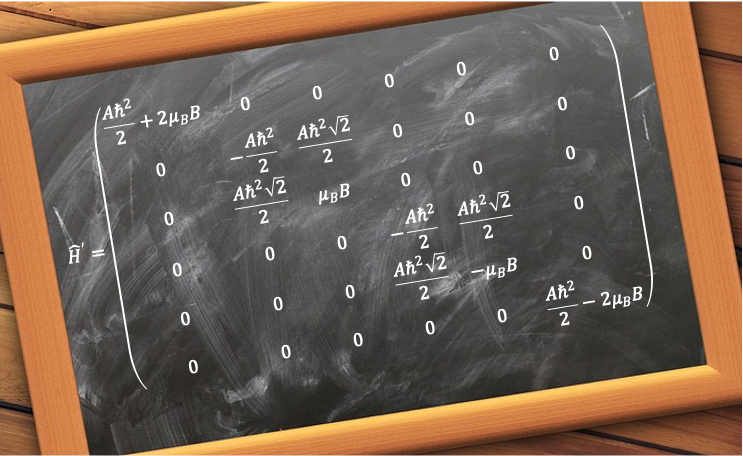
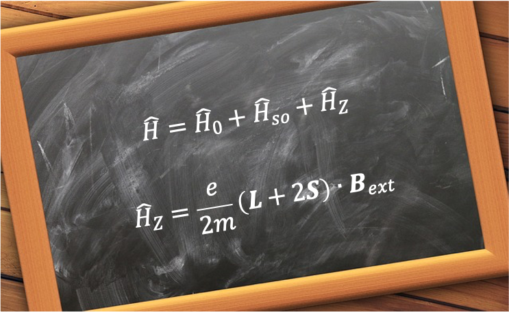
It is defined as the first-order energy correction in perturbation theory and is most clearly observed in hydrogenic atoms, where the high symmetry of the Coulomb potential leads to degeneracies that allow first-order shifts. In the strong-field regime ( $E\geq 10^7$ V/m), where the static, uniform electric field strength $\boldsymbol{\mathit{E}}$ produces energy shifts that are large compared to those arising from spin-orbit interactions, the Hamiltonian $\hat{H}$ for a hydrogenic atom is:

$\hat{H}=\hat{H}_0+\hat{H}_S\;\;\;\;\;\;\;\;360$

where $\hat{H}_0$ is the Hamiltonian of the unperturbed atom and $\hat{H}_S$ is the perturbation due to the Stark effect.

The perturbing Hamiltonian is given by eq354:

$\hat{H}_S=-\hat{\boldsymbol{\mathit{\mu}}}\cdot\boldsymbol{\mathit{E}}$

where $\hat{\boldsymbol{\mathit{\mu}}}$ is the operator of the electric dipole moment of the atom.

This suggests that $\hat{H}_S$ vanishes if the electric dipole operator is zero. Substituting eq350 into $\hat{H}_S$ gives

$\hat{H}_S=e\hat{\boldsymbol{\mathit{r}}}\cdot\boldsymbol{\mathit{E}}\;\;\;\;\;\;\;\;361$

where $\hat{\boldsymbol{\mathit{r}}}$ is the operator of the position vector $\boldsymbol{\mathit{r}}$ of the electron, with the vector measured from the nucleus (taken as the origin).

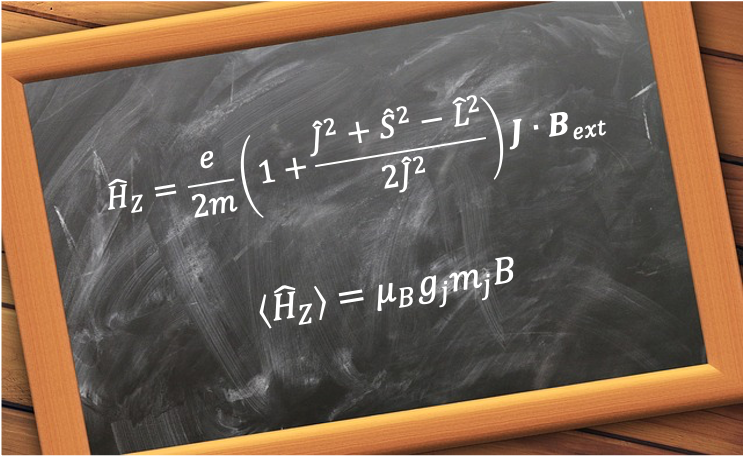
Compared to the Zeeman Hamiltonian, which depends on both the orbital and spin angular momenta of the electron, the Stark Hamiltonian depends only on $\boldsymbol{\mathit{r}}$ and therefore acts only on the spatial part of the hydrogenic wavefunction.

Assuming that the electric field is directed along the laboratory $z$ -axis, eq361 becomes

$\hat{H}_S=ezE=eErcos\theta\;\;\;\;\;\;\;\;362$

where $\theta$ is the angle between $\boldsymbol{\mathit{r}}$ and the $z$ -axis.

To understand how the perturbation affects the energy levels, we analyse its effect on the $n=1$ and $n=2$ states of the atom. The uncoupled wavefunction $\vert n,l,m_l\rangle$ , which is a good eigenstate of $\hat{H}_0$ , is used as a basis to begin the perturbation analysis. For $n=1$ , the eigenstate $\psi=\vert n,l,m_l\rangle$ is the non-degenerate ground state $\vert 1,0,0\rangle=\frac{1}{\sqrt{\pi a^3_0}}e^{-\frac{r}{a_0}}$ . Therefore, we may apply the first-order non-degenerate perturbation theory, which corresponds to the expectation value of $\hat{H}_S$ :

$E_1^{(1)}=\langle 1,0,0\vert\hat{H}_S\vert 1,0,0\rangle$

or equivalently, in spherical coordinates,

$E_1^{(1)}=\frac{eE}{\pi a^3_0}\int e^{-\frac{2r}{a_0}}rcos\theta r^2sin\theta drd\theta d\phi\;\;\;\;\;\;\;\;363$

Since $\int^{\pi}_0cos\theta sin\theta d\theta=0$ , we have $E_1^{(1)}=0$ . Therefore, the ground state of a hydrogenic atom exhibits no first-order Stark effect, as its spherical symmetry implies that it possesses no permanent electric dipole moment. In fact, because $r$ is odd under spatial inversion (it changes sign about the origin), its expectation value vanishes for any eigenstate of even parity, since the integral of an odd function multiplied by an even function over all space is zero.

Unlike the ground state, the unperturbed $n=2$ level is fourfold degenerate described by the following basis wavefunctions (see this article and this article for derivation):

$\psi_{2s}=\vert 2,0,0\rangle=\frac{1}{4\sqrt{2\pi}}\sqrt{\biggr$\frac{1}{a_0}\biggr$^3}\biggr$2-\frac{r}{a_0}\biggr$e^{-\frac{r}{2a_0}}$

$\psi_{2p_z}=\vert 2,1,0\rangle=\frac{1}{4\sqrt{2\pi}}\sqrt{\biggr$\frac{1}{a_0}\biggr$^5}e^{-\frac{r}{2a_0}}rcos\theta$

$\vert 2,1,1\rangle=\frac{1}{8\sqrt{\pi}}\sqrt{\biggr$\frac{1}{a_0}\biggr$^5}re^{-\frac{r}{2a_0}}(1-cos^2\theta)^{1/2}e^{i\phi}$

$\vert 2,1,-1\rangle=\frac{1}{8\sqrt{\pi}}\sqrt{\biggr$\frac{1}{a_0}\biggr$^5}re^{-\frac{r}{2a_0}}(1-cos^2\theta)^{1/2}e^{-i\phi}$

Due to this degeneracy, we must use degenerate perturbation theory, which requires constructing the $4\times 4$ Stark Hamiltonian matrix with elements $\langle\psi_i\vert\hat{H}_S\vert\psi_j\rangle$ . Because $\psi^*_i\psi_i=\vert\psi_i\vert^2$ has even parity and $\hat{H}_S\propto r$ is odd under spatial inversion, all diagonal matrix elements vanish:

$\langle 2,0,0\vert\hat{H}_S\vert 2,0,0\rangle=0$

$\langle 2,1,0\vert\hat{H}_S\vert 2,1,0\rangle=0$

$\langle 2,1,1\vert\hat{H}_S\vert 2,1,1\rangle=0$

$\langle 2,1,-1\vert\hat{H}_S\vert 2,1,-1\rangle=0$

Furthermore, the matrix elements $\langle 2,0,0\vert\hat{H}_S\vert 2,1,1\rangle$ , $\langle 2,0,0\vert\hat{H}_S\vert 2,1,-1\rangle$ , $\langle 2,1,1\vert\hat{H}_S\vert 2,1,0\rangle$ , $\langle 2,1,1\vert\hat{H}_S\vert 2,1,-1\rangle$ and $\langle 2,1,0\vert\hat{H}_S\vert 2,1,-1\rangle$ , together with their complex conjugates, are all zero because their corresponding azimuthal integrals involve terms such as $\int_0^{2\pi}e^{i\phi}d\phi$ , $\int_0^{2\pi}e^{-i\phi}d\phi$ or $\int_0^{2\pi}e^{-2i\phi}d\phi$ , all of which vanish. This leaves $\langle 2,0,0\vert\hat{H}_S\vert 2,1,0\rangle$ and its complex conjugate $\langle 2,1,0\vert\hat{H}_S\vert 2,0,0\rangle$ , each of which evaluates to $-3a_0eE$ .

Question

Show that $\langle 2,0,0\vert\hat{H}_S\vert 2,1,0\rangle=-3a_0eE$

Answer

$\langle 2,0,0\vert\hat{H}_S\vert 2,1,0\rangle=\frac{eE}{32\pi a_0^4}\int_0^{\infty}\biggr$2-\frac{r}{a_0}\biggr$e^{-\frac{r}{a_0}}r^4dr\int_0^{\pi}cos^2\theta sin\theta d\theta\int_0^{2\pi}d\phi$

Letting $u=cos\theta$ , $du=-sin\theta d\theta$ , we have $\int_0^{\pi}cos^2\theta sin\theta d\theta=\int_{-1}^1u^2du=\frac{2}{3}$ , and

$\langle 2,0,0\vert\hat{H}_S\vert 2,1,0\rangle=\frac{eE}{12 a_0^4}\int_0^{\infty}r^4e^{-\frac{r}{a_0}}dr-\frac{1}{24a_0^5}\int_0^{\infty}r^5e^{-\frac{r}{a_0}}dr$

Using the identity $\int_0^{\infty}x^me^{-ax}dx=\frac{m!}{a^{m+1}}$ completes the maths.

Therefore, we need to solve the eigenvalue equation

$\hat{H}_S\begin{pmatrix}c_1\\c_2\\c_3\\c_4\end{pmatrix}=\lambda\begin{pmatrix}c_1\\c_2\\c_3\\c_4\end{pmatrix}\;\;\;\;\;\;\;\;364$

where $c_1$ , $c_2$ , $c_3$ and $c_4$ are the coefficients in the basis $\{\vert2,0,0\rangle,\vert2,1,1\rangle,\vert2,1,0\rangle,\vert2,1,-1\rangle,$ and

$\hat{H}_S=-3a_0eE\begin{pmatrix}0&0&1&0\\0&0&0&0\\1&0&0&0\\0&0&0&0\end{pmatrix}$

To find the eigenvalues, we solve the secular equation $\vert\hat{H}_S-\lambda I\vert=0$ or equivalently,

$\begin{vmatrix}-\lambda&0&-3a_0eE&0\\0&-\lambda&0&0\\-3a_0eE&0&-\lambda&0\\0&0&0&-\lambda\end{vmatrix}=0$

Evaluating the determinant gives the characteristic equation:

$\lambda^4-(3a_0eE)^2\lambda^2=0$

with solutions:

$\lambda=E_2^{(1)}=0,0,+3a_0eE,-3a_0eE\;\;\;\;\;\;\;\;365$

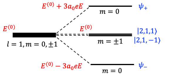
Therefore, the fourfold degenerate $n=2$ level is split by the Stark effect into three distinct levels (see diagram below): $E^{(0)}$ , $E^{(0)}+3a_0eE$ and $E^{(0)}-3a_0eE$ , where $E^{(0)}$ is the eigenvalue of the unperturbed Hamiltonian $\hat{H}_0$ .

To determine the eigenstates corresponding to the three distinct levels, we refer to eq364, where

$\hat{H}_S\begin{pmatrix}c_1\\c_2\\c_3\\c_4\end{pmatrix}=\begin{pmatrix}-3a_0eEc_3\\0\\-3a_0eEc_1\\0\end{pmatrix}=\lambda\begin{pmatrix}c_1\\c_2\\c_3\\c_4\end{pmatrix}\;\;\;\;\;\;\;\;366$

For $\lambda=0$ , we require $c_3=0$ and $c_1=0$ . Since there are no conditions on $c_2$ or $c_4$ , any linear combination of $\vert 2,1,1\rangle$ and $\vert 2,1,-1\rangle$ is an eigenstate with eigenvalue 0. However, a state $\psi=c_2\vert 2,1,1\rangle+c_4\vert 2,1,-1\rangle$ , with both $c_2\neq 0$ and $c_4\neq 0$ , is not an eigenstate of $\hat{l}_z$ (i.e. $m_l$ is not well-defined). Therefore, only the linear combinations in which either $c_2=0$ or $c_4=0$ , namely the unmixed states $\vert 2,1,1\rangle$ or $\vert 2,1,-1\rangle$ , are good eigenstates of both $\hat{H}$ and $\hat{l}_z$ for $\lambda=0$ .

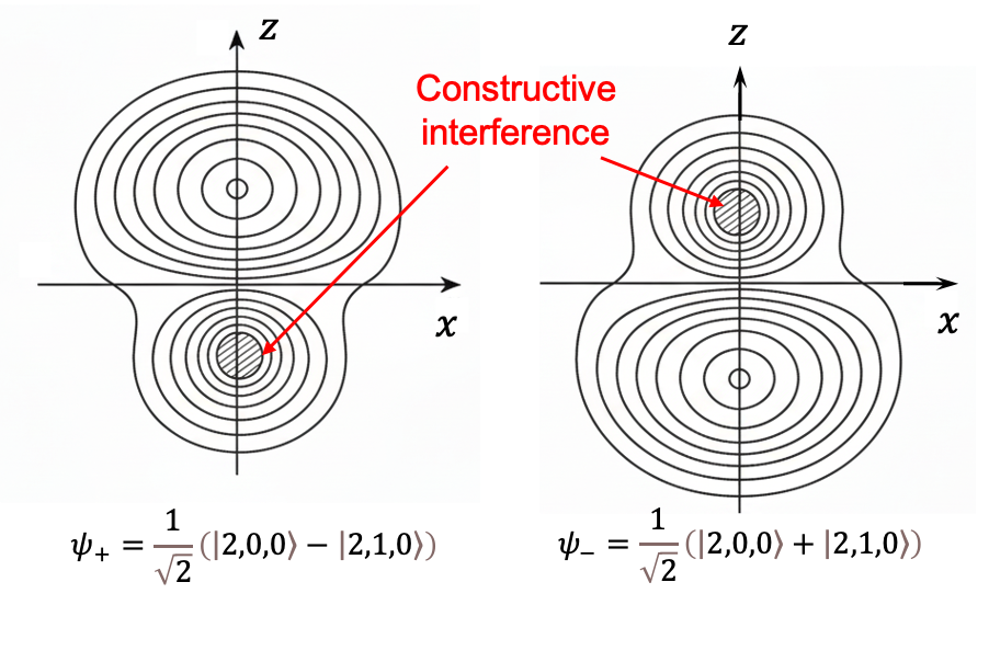
For $\lambda=+3a_0eE$ , eq366 gives the condition $c_1=-c_3$ and $c_2=c_4=0$ . Hence, the normalised eigenstate is

$\psi_+=\frac{1}{\sqrt{2}}(\vert 2,0,0\rangle-\vert 2,1,0\rangle)$

Similarly, for $\lambda=-3a_0eE$ , the same equation yields $c_1=c_3$ and $c_2=c_4=0$ resulting in the normalised eigenstate

$\psi_-=\frac{1}{\sqrt{2}}(\vert 2,0,0\rangle+\vert 2,1,0\rangle)$

Since both $\vert 2,0,0\rangle$ and $\vert 2,1,0\rangle$ are eigenstates of $\hat{l}_z$ , each with eigenvalue $0$ , $\psi_+$ and $\psi_-$ remain eigenstates of $\hat{l}_z$ . However, $\psi_+$ and $\psi_-$ are no longer eigenstates of $\hat{L}^2$ , meaning $l$ is not a good quantum number once the electric field is applied.

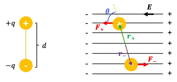
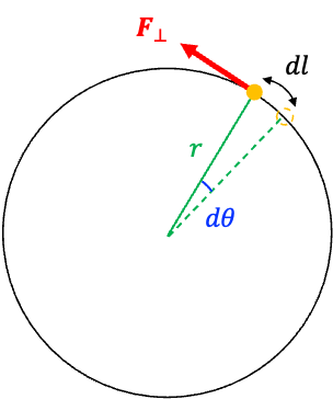
The fact that the $n=2$ level exhibits a first-order Stark effect for $\psi_+$ and $\psi_-$ implies that their electron distributions are no longer spherically symmetric and acquire a permanent electric dipole moment along the field direction (see diagram below). Furthermore, the three distinct energy levels, $-3a_0eE$ , $0$ and $+3a_0eE$ , classically suggest that the dipole moment has magnitude $3a_0e$ and three possible orientations: parallel, antiparallel and perpendicular to the field.

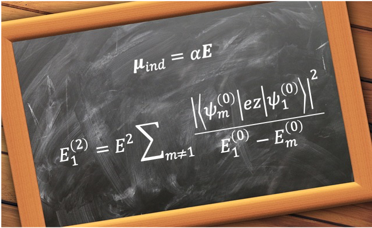
Because the Stark energy shifts in hydrogenic atoms are proportional to the first power of the electric field, the phenomenon is known as the linear Stark effect. Although the ground state of hydrogen does not exhibit a linear Stark effect, it does exhibit a quadratic Stark effect, which we will explore in the next article.

Next article: Quadratic Stark effect

Previous article: Stark effect

Content page of quantum mechanics

Content page of advanced chemistry

Main content page

March 2, 2026April 4, 2026

Quadratic Stark effect

The quadratic Stark effect is the shift of atomic or molecular energy levels proportional to the square of an applied electric field, arising when non-degenerate states produce only second-order energy corrections.

As explained in the previous article, the ground state ( $n=1$ ) of hydrogen does not exhibit a linear Stark effect, which is defined as the first-order energy correction in perturbation theory, because its spherical symmetry implies that it possesses no permanent electric dipole moment. With reference to eq270a, the second-order energy correction for the ground state of hydrogen $E_1^{(2)}$ is

$E_1^{(2)}=\langle\psi_1^{(0)}\vert\hat{H}^{(1)}\vert\Psi_1^{(1)}\rangle=\sum_{m\neq 1}\frac{\vert\langle\psi_m^{\;(0)}\vert\hat{H}_S\vert\psi_1^{\;(0)}\rangle\vert^2}{E_1^{\;(0)}-E_m^{\;(0)}}\;\;\;\;\;\;\;\;370$

where
$\hat{H}_S=eEz$ is the perturbing part of the Hamiltonian due to the Stark effect (see eq362)
$E$ is the external electric field directed along the $z$ -axis
$\Psi_1^{(1)}=\sum_{m\neq 1}c_m\psi_m^{(0)}$ is a linear combination (mixing) of excited eigenstates, with $c_m$ given by eq269a
$\psi_1^{(0)}$ and $E_1^{(0)}$ are the ground state eigenfunction and eigenvalue
$\psi_m^{(0)}$ and $E_m^{(0)}$ are the eigenfunctions and eigenvalues for $n>1$ .

Since $\psi_1^{(0)}$ corresponds to the 1s wavefunction, which is an even function under spatial inversion, and $z$ is odd under spatial inversion, $\hat{H}_S\psi_1^{(0)}$ is an odd function. Consequently, for $\langle\psi_m^{(0)}\vert\hat{H}_S\vert\psi_1^{(0)}\rangle\neq 0$ , $\psi_m^{(0)}$ must be odd. The term in the summation with the smallest magnitude of the denominator $E_1^{(0)}-E_m^{(0)}$ contributes most significantly to $E_1^{(2)}$ . This occurs when $m=2$ , implying that the 2p wavefunctions $\psi_{m=2}^{(0)}$ (which are the only odd-parity states in the $n=2$ level) dominate the correction to the eigenvalue.

It follows that the ground state of hydrogen exhibits a Stark effect when the second-order energy correction is taken into account. To show that it is a quadratic effect and that the associated electric dipole moment is an induced dipole moment, we substitute eq362 into eq370 to obtain

$E_1^{(2)}=E^2\sum_{m\neq 1}\frac{\vert\langle\psi_m^{\;(0)}\vert ez\vert\psi_1^{\;(0)}\rangle\vert^2}{E_1^{\;(0)}-E_m^{\;(0)}}\;\;\;\;\;\;\;\;371$

Clearly, the second-order energy correction is proportional to $E^2$ , and hence represents a quadratic Stark effect.

In classical electromagnetism, the energy of an electric dipole moment in an external field is given by eq354, or in differential form:

$dE_1^{(2)}=-\boldsymbol{\mathit{\mu}}\cdot d\boldsymbol{\mathit{E}}$

Substituting the definition of an induced electric dipole moment $\boldsymbol{\mathit{\mu}}_{ind}=\alpha\boldsymbol{\mathit{E}}$ into $dE_1^{(2)}$ gives

$dE_1^{(2)}=-\alpha\boldsymbol{\mathit{E}}\cdot d\boldsymbol{\mathit{E}}$

Since the external electric field is directed along the $z$ -axis,

$E_1^{(2)}=-\alpha\int_0^EEdE=-\frac{1}{2}\alpha E^2\;\;\;\;\;\;\;\;372$

If $E_1^{(2)}$ in eq371 is an energy shift arising from an induced dipole moment, it must have the form of given in eq372. Comparing eq371 with eq372 yields

$\alpha=2\sum_{m\neq 1}\frac{\vert\langle\psi_m^{\;(0)}\vert ez\vert\psi_1^{\;(0)}\rangle\vert^2}{E_m^{\;(0)}-E_1^{\;(0)}}$

where $\alpha$ is the polarisability of the atom, which is a measure of the degree to which the electron in hydrogen can be displaced relative to the nucleus.

Therefore, $E_1^{(2)}$ in eq371 is an energy shift arising from an induced dipole moment. Even though the ground state of hydrogen does not possess a permanent dipole moment, it exhibits a quadratic Stark effect due to the electric dipole moment induced by an external electric field.

NExt article: Inductive effect

Previous article: Linear Stark effect

Content page of quantum mechanics

Content page of advanced chemistry

Main content page

February 25, 2026March 2, 2026

Stark effect

The Stark effect is the shifting and splitting of atomic or molecular spectral lines when an external electric field is applied.

First observed in 1913 by Johannes Stark, this phenomenon provided important early evidence for the interaction between electromagnetic fields and atomic structure. The effect arises because the electric field perturbs the energy levels of electrons, altering the frequencies of light emitted or absorbed during electronic transitions. As the electric analogue of the Zeeman effect, the Stark effect is analysed using perturbation theory and plays a significant role in spectroscopy and quantum mechanics.

The precise way in which these spectral lines shift, however, depends on both the internal structure of the atom or molecule and the strength of the applied electric field. In practice, two principal regimes are distinguished: the linear Stark effect and the quadratic Stark effect.

The linear Stark effect is defined as the first-order energy correction in perturbation theory and occurs when the energy shift is directly proportional to the strength of the applied electric field. This behaviour typically appears in systems with degenerate energy levels, such as in the hydrogen atom. In contrast, the quadratic Stark effect corresponds to the second-order energy correction and occurs when the energy shift is proportional to the square of the electric field strength. This is the more common situation for atoms and molecules with non-degenerate energy levels.

Details of these two effects will be discussed in the next two articles.

Next article: Linear Stark effect

Previous article: Electric dipole moment

Content page of quantum mechanics

Content page of advanced chemistry

Main content page

February 10, 2026February 25, 2026

Electric dipole moment

An electric dipole is a pair of equal and opposite electric charges, $+q$ and $-q$ , separated by a small distance $d$ . The electric dipole moment $\boldsymbol{\mathit{\mu}}$ (also denoted by $\boldsymbol{\mathit{p}}$ ) is a measure of the strength and orientation of the electric dipole and is defined as:

$\boldsymbol{\mathit{\mu}}=\sum_iq_i\boldsymbol{\mathit{r}}_i=(+q)\frac{\boldsymbol{\mathit{d}}}{2}+(-q)\biggr$-\frac{\boldsymbol{\mathit{d}}}{2}\biggr$=q\boldsymbol{\mathit{d}}\;\;\;\;\;\;\;\;350$

where $\boldsymbol{\mathit{r}}_i$ is the position vector of the corresponding charge measured from the origin, which is usually taken at the midpoint between the charges.

The SI unit of electric dipole moment is the Coulomb-meter (C·m), although the Debye (D) is more commonly used in practice (1D » 3.33 x 10^-30 C·m)

Question

Is the electric dipole a vector?

Answer

The electric dipole is a physical configuration of two equal and opposite charges, not a vector. However, the associated electric dipole moment is a vector quantity. By physics convention, its direction points from the negative charge to the positive charge (note that in chemistry, the dipole direction is taken from the less electronegative atom to the more electronegative atom).

When an electric dipole is placed in an external electric field $\boldsymbol{\mathit{E}}$ (see diagram above), it experiences a torque $\boldsymbol{\mathit{\tau}}$ that tends to rotates the dipole so as to align it with the field, thereby lowering its potential energy. The torque is defined as the product of the component of a force $F_{\perp}$ normal to the axis of rotation and the distance $r$ from the origin to the point of application of the force ( $\tau=rF_{\perp}=rFsin\theta$ or equivalently $\boldsymbol{\mathit{\tau}}=\boldsymbol{\mathit{r}}\times\boldsymbol{\mathit{F}}$ ). For a spatially uniform electric field,

$\begin{align}\boldsymbol{\mathit{\tau}}&=\sum_i(\boldsymbol{\mathit{r}}_i\times\boldsymbol{\mathit{F}}_i)=\frac{\boldsymbol{\mathit{d}}}{2}\times\boldsymbol{\mathit{F}}_++\biggr$-\frac{\boldsymbol{\mathit{d}}}{2}\biggr$\times\boldsymbol{\mathit{F}}_-\\&=\frac{\boldsymbol{\mathit{d}}}{2}\times(+q\boldsymbol{\mathit{E}})+\biggr$-\frac{\boldsymbol{\mathit{d}}}{2}\biggr$\times(-q\boldsymbol{\mathit{E}})=\boldsymbol{\mathit{\mu}}\times\boldsymbol{\mathit{E}}\;\;\;\;\;\;\;\;351\end{align}$

$\boldsymbol{\mathit{E}}$ and $\boldsymbol{\mathit{\mu}}$ define a plane, and $\boldsymbol{\mathit{\tau}}$ is perpendicular to this plane, with its direction given by the right-hand rule. Therefore, the magnitude of the torque is

$\tau=\mu Esin\theta\;\;\;\;\;\;\;\;352$

where $\theta$ is the angle between the rotating axis and the force, which is equivalent to the angle between $\boldsymbol{\mathit{\mu}}$ and $\boldsymbol{\mathit{E}}$ .

For a rotating system (see diagram above), the work done $W$ is given by

$W=\int F_{\perp}dl$

Since $dl=rd\theta$ and the change in potential energy $U$ is the negative of the work done by the field,

$U_f-U_i=-\int^{\theta_f}_{\theta_i}F_{\perp}rd\theta=-\int^{\theta_f}_{\theta_i}\tau d\theta\;\;\;\;\;\;\;\;353$

Substituting eq352 into eq353 yields:

$U_f-U_i=-\int^{\theta_f}_{\theta_i}\mu Esin\theta d\theta=\mu E(cos\theta_f-cos\theta_i)$

Because the force exerted by the electric field rotates the dipole towards a lower potential energy, $U_f-U_i<0$ . To satisfy this condition, as $\theta$ changes from $90^{\circ}$ to $0^{\circ}$ during the rotation, we define $U_i=0$ when the dipole is perpendicular to the field ( $\theta_i=90^{\circ}$ ), giving

$U=-\mu Ecos\theta$

where $U_f=U$ and the negative sign arises naturally to ensure that $U<0$ ( $cos\theta$ is positive for $0^{\circ}\leq\theta_f=\theta<90^{\circ}$ ), with the corresponding potential energy in vector form being

$U=-\boldsymbol{\mathit{\mu}}\cdot\boldsymbol{\mathit{E}}\;\;\;\;\;\;\;\;354$

The electric dipole moment is used to determine electronic transition probabilities in atoms and molecules.

Question

Answer

next article: Electrolysis of water

Previous article: lithium-ion battery

Next article: Mesomeric effect

Previous article: Linear Stark effect

Question

Answer

Question

Answer

Question

Answer

Next article: Ortho/Para and meta directing groups

Previous article: Inductive effect

Question

Answer

Previous article: Mesomeric effect

Question

Answer

Next article: Why does a current flowing through a wire generate a magnetic field

Previous article: Length contraction

Next article: Overlap integral

Previous article: The variational method

Question

Answer

Next article: Quadratic Stark effect

Previous article: Stark effect

NExt article: Inductive effect

Previous article: Linear Stark effect

Next article: Linear Stark effect

Previous article: Electric dipole moment

Question

Answer

Next article: Stark effect

Previous article: Intermediate-field case of the Zeeman effect