Laguerre polynomials are a sequence of polynomials that are solutions to the Laguerre differential equation:
where is a constant.

When , eq420 simplifies to
. The solution to this first-order differential equation is
, which can be expressed as the Taylor series
. This implies that eq420 has a power series solution around
. To determine the exact form of the power series solution to eq420, let
.
Substituting ,
and
in eq420 yields
Setting in the first sum,
Eq422 is only true if all coefficients of in is 0 (see this article for explanation). So,
, or equivalently,
Eq423 is a recurrence relation. If we know the value of , we can use the relation to find
.
| Recurrence relation | |
Comparing the recurrence relations, we have
where by convention (so that
).
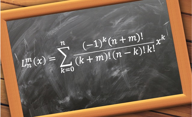
Letting in eq424 and substituting it in
yields the Laguerre polynomials:
where we have replaced with
.
The first few Laguerre polynomials are: