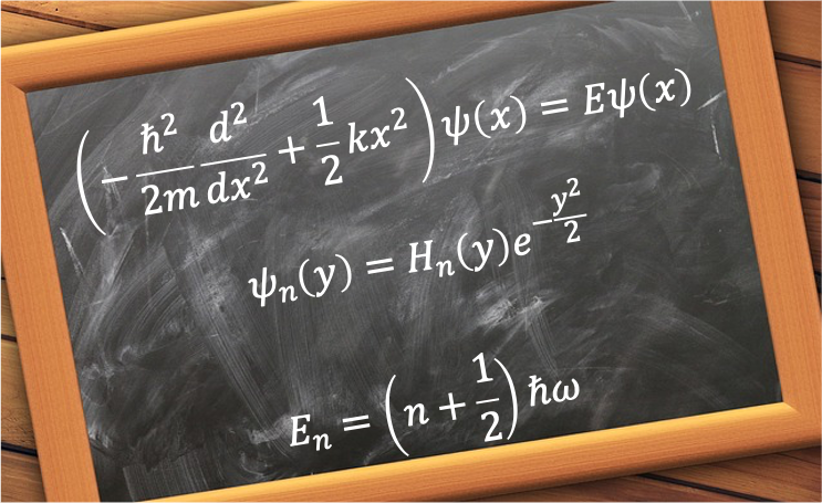
The quantum harmonic oscillator is a model for studying an atom that moves back and forth about an equilibrium point. The model’s central premise involves the use of the potential energy term of the classical harmonic oscillator to construct the Schrodinger equation for the harmonic oscillator:
\psi(x)=E\psi(x)\;\;\;\;\;\;\;\;4)
which is equivalent to
\psi(x)=E\psi(x))
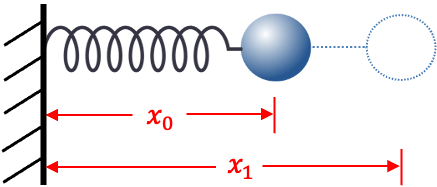
where  is the displacement of the mass from its equilibrium position.
Substituting  in the above equation and rearranging, we have
+\biggr\(\frac{2m}{\hbar^2}E-\frac{m^2\omega^2}{\hbar^2}\biggr\)\psi(x)=0\;\;\;\;\;\;\;\;5)
The probability of locating an electron in the Hilbert space must be finite, i.e. \vert^2dx<\infty) . This implies that
. This implies that ) vanishes as
vanishes as  . We call such a well-behaved wavefunction square-integrable. Hence, we need to study the asymptotic characteristics of eq5 to find possible solutions.
Let’s begin by simplifying the differential equation using a change of variable. Substituting ^{1/2}) and
and  in eq5, we have
}{dy^2}+\(2\epsilon-y^2)\psi(y)=0\;\;\;\;\;\;\;\;6)
Since  is a constant,
  as
as  , and eq6 approximates to
}{dy^2}-y^2\psi(y)=0\;\;\;\;\;\;\;\;7)
This suggests that the solution to eq6 could be a Gaussian function because =e^{-\frac{y^2}{2}}) is a solution to eq7. Let’s try
is a solution to eq7. Let’s try =u(y)e^{-\frac{y^2}{2}}) , where
, where ) is a function of
is a function of  . Substituting in eq6 and computing the derivatives, we have
}{dy^2}-2y\frac{du(y)}{dy}+(2\epsilon-1)u(y)=0\;\;\;\;\;\;\;\;8)
Eq8 is known as the Hermite differential equation.
The above Q&A suggests that a possible solution to eq8 is a power series for a range of values of . Let =\sum_{n=0}^{\infty}C_ny^n) and substitute
and substitute }{dy}=\sum_{n=0}^{\infty}nC_ny^{n-1}) and
and }{dy^2}=\sum_{n=0}^{\infty}n(n-1)C_ny^{n-2}) in eq8 to give
in eq8 to give
C_ny^{n-2}-2y\sum_{n=0}^{\infty}nC_ny^{n-1}+(2\epsilon-1)\sum_{n=0}^{\infty}C_ny^{n}=0)
Substituting  and
and C_ny^{n-2}=\sum_{n=0}^{\infty}(n+2)(n+1)C_{n+2}y^n) in the above equation, we have
in the above equation, we have
(n+1)C_{n+2}-2nC_n+(2\epsilon-1)C_n\]y^n=0)
The above equation is only true for all values of if every coefficient for each power of is zero. So, (n+1)C_{n+2}-2nC_n+(2\epsilon-1)C_n=0) , which rearranges to
, which rearranges to
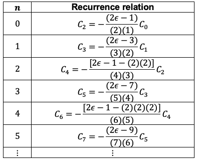
(n+1)}C_n\;\;\;\;\;\;\;\;9)
Eq9 is a recurrence relation. If we know the value of  , we can use the relation to find
  . Similarly, if we know
  , we can find
  .
.
Comparing the recurrence relations for even-labelled coefficients,
\]\frac{(2n-2)!}{(2n)!}C_{2n-2}\;\;\;where\;n=1,2,3\cdots\;\;\;\;10)
Similarly, the recurrence relations for odd-labelled coefficients can be expressed as
\]\frac{(2n-1)!}{(2n+1)!}C_{2n-1}\;\;\;where\;n=1,2,3\cdots\;\;\;\;11)
Rewriting ) as a sum of two power series, one containing terms with even-labelled coefficients and the other with odd-labelled coefficients,
as a sum of two power series, one containing terms with even-labelled coefficients and the other with odd-labelled coefficients,
=\biggr\{C_0+\sum_{l=1}^{\infty}\biggr\[-\[2\epsilon-1-2(2l-2)\]\frac{C_{2l-2}}{\frac{(2l)!}{(2l-2)!}}\biggr\]y^{2l}\biggr\}e^{-\frac{y^2}{2}}+\\\biggr\{C_1y+\sum_{l=1}^{\infty}\biggr\[-\[2\epsilon-3-2(2l-2)\]\frac{C_{2l-1}}{\frac{(2l+1)!}{(2l-1)!}}\biggr\]y^{2l+1}\biggr\}e^{-\frac{y^2}{2}}\;\;\;\;\;\;\;\;12)
According to L’Hopital’s rule, appears to be a possible solution to eq7 because each of the terms in eq12 (simplified to  ) approaches zero for large :

where  is a constant.
However, this does not guarantee that the series as a whole also converges because the sum of an infinite number of infinitesimal terms can still be infinite, as is the case for a harmonic series. To see how the two infinite series behave for large , we carry out the ratio test as follows:

where we have set  and
and  in eq9 for the even series and odd series respectively.
By comparison, the ratio test for the power series expansion of  is also
  . Therefore, both infinite series behave the same as
  and diverge for large . To ensure that is square-integrable, we need to truncate either one of the series after some finite terms
  and let all the coefficients of the other series be zero.
To truncate either series, we let the numerator of eq9 be zero so that every successive term in the selected series is zero as well. This implies that

Let’s rewrite eq12 as
=\biggr\{\begin{matrix}\biggr\{C_0+\sum_{l=1}^{m}\biggr\[-\[2\epsilon-1-2(2l-2)\]\frac{C_{2l-2}}{\frac{(2l)!}{(2l-2)!}}\biggr\]y^{2l}\biggr\}e^{-\frac{y^2}{2}}&even\;series\;l=1,2,\cdots\\\biggr\{C_1y+\sum_{l=1}^{m}\biggr\[-\[2\epsilon-3-2(2l-2)\]\frac{C_{2l-1}}{\frac{(2l+1)!}{(2l-1)!}}\biggr\]y^{2l+1}\biggr\}e^{-\frac{y^2}{2}}&odd\;series\;l=1,2,\cdots\end{matrix}\;\;\;\;14)
Since eq14 is the result of substituting in eq6, it is a solution to eq6.

Question
Show that =C_0\biggr\[1-\frac{2n}{2!}y^2+\frac{2^2n(n-2)}{4!}y^4\biggr\]e^{-\frac{y^2}{2}}) .
.
Answer
We expand the even series in eq14 as follows:
=\biggr\[C_0-(2\epsilon-1)\frac{C_0}{2!}y^2-2(2\epsilon-1-4)\frac{C_2}{4!}y^4\biggr\]e^{-\frac{y^2}{2}})
Substituting eq9, where  , in the above equation, we have
=\biggr\[C_0-(2\epsilon-1)\frac{C_0}{2!}y^2-\frac{(2\epsilon-1-4)(1-2\epsilon)}{4!}C_0y^4\biggr\]e^{-\frac{y^2}{2}})
Substituting eq13 in the above equation gives the required expression.
Re-expanding the even series of eq14 using eq9 and eq13, we have
Comparing the coefficients of each even series in the above table, we have
=C_0\biggr\[1-\frac{2n}{2!}y^2+\frac{2^2n(n-2)}{4!}y^4+\cdots+\frac{2^n\(\frac{n}{2}\)!}{(-1)^{\frac{n}{2}}n!}y^n\biggr\]e^{-\frac{y^2}{2}}\;\;\;\;\;\;\;\;15a)
where  .
.
Similarly, the re-expansion of the odd series of eq14 using eq9 and eq13 gives
Comparing the coefficients of each odd series in the above table, we have
=C_1\biggr\[y-\frac{2(n-1)}{3!}y^3+\frac{2^2(n-1)(n-3)}{5!}y^5+\cdots+\frac{2^n\(\frac{n-1}{2}\)!}{(-1)^{\frac{n-1}{2}}2(n!)}y^n\biggr\]e^{-\frac{y^2}{2}}\;\;\;\;\;\;\;\;15b)
where  .
.
The recurrence relation of eq9 that led to eq14 only defines the value of  in terms of
  . This implies that there are many solution sets depending on the value of . The convention is to set the leading coefficients (i.e. the coefficients of
  ) of eq15a and eq15b, which are independent of each other, as
  . Therefore,
!}{(-1)^{\frac{n}{2}}n!}=2^n\;\;or\;\;C_0=(-1)^{\frac{n}{2}}\frac{n!}{(\frac{n}{2})!}\;\;\;\;\;\;\;\;16)
and
!}{(-1)^{\frac{n-1}{2}}2(n!)}=2^n\;\;or\;\;C_1=(-1)^{\frac{n-1}{2}}\frac{2(n!)}{(\frac{n-1}{2})!}\;\;\;\;\;\;\;\;17)
Substituting eq16 and eq17 in eq14, we have =H_n(y)e^{-\frac{y^2}{2}}) , where
, where ) are the Hermite polynomials:
are the Hermite polynomials:
=\biggr\{\begin{matrix}\biggr\{(-1)^{\frac{n}{2}}\frac{n!}{(\frac{n}{2})!}+\sum_{l=1}^{m}\biggr\[-\[2\epsilon-1-2(2l-2)\]\frac{C_{2l-2}}{\frac{(2l)!}{(2l-2)!}}\biggr\]y^{2l}\biggr\}e^{-\frac{y^2}{2}}&even\;series\;l=1,2,\cdots\\\biggr\{(-1)^{\frac{n-1}{2}}\frac{2(n!)}{(\frac{n-1}{2})!}y+\sum_{l=1}^{m}\biggr\[-\[2\epsilon-3-2(2l-2)\]\frac{C_{2l-1}}{\frac{(2l+1)!}{(2l-1)!}}\biggr\]y^{2l+1}\biggr\}e^{-\frac{y^2}{2}}&odd\;series\;l=1,2,\cdots\end{matrix}\;\;\;\;18)
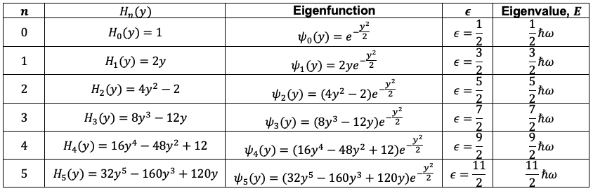
The first few Hermite polynomials, un-normalised eigenfunctions of eq6 and their corresponding eigenvalues are
When  , we can express the Hermite polynomials for odd
  as
as
=0\;\;\;n=0,1,2,\cdots\;\;\;\;\;\;\;\;19)
Similarly, when , we can express the Hermite polynomials for even as
=\frac{(-1)^n(2n)!}{n!}\;\;\;n=0,1,2,\cdots\;\;\;\;\;\;\;\;20)
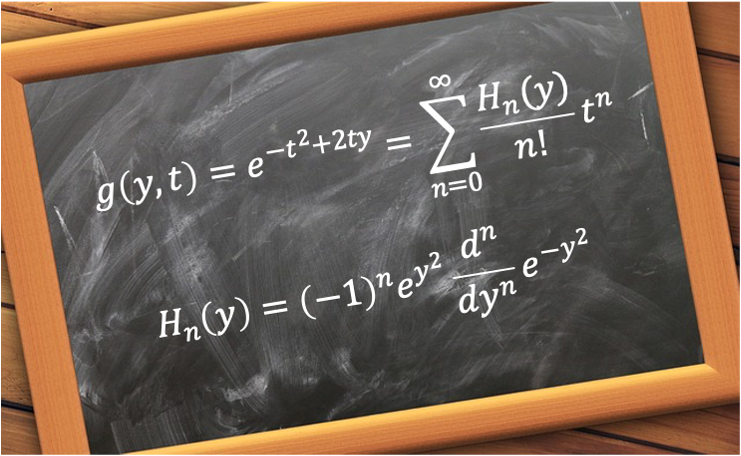
Eq19 and eq20 are useful in proving the generating function for Hermite polynomials.
The table above also shows that the energy states  of a quantum-mechanical harmonic oscillator are quantised:
\hbar\omega\;\;\;n=0,1,2,\cdots\;\;\;\;\;21)
with the ground state  being non-zero. This energy is called the zero-point energy of the harmonic oscillator.
Since is a solution to eq8, we can rewrite eq8 as
}{dy^2}-2y\frac{dH_n(y)}{dy}+(2\epsilon-1)H_n(y)=0\;\;\;\;\;\;\;\;22)
To complete the prove that =H_n(y)e^{-\frac{y^2}{2}}) is a solution to eq6, we will derive the normalisation constant
is a solution to eq6, we will derive the normalisation constant  of
of =N_nH_n(y)e^{-\frac{y^2}{2}}) and prove that the wavefunctions are orthogonal to one another in the next few articles.
and prove that the wavefunctions are orthogonal to one another in the next few articles.
Question
Do we have to change the variable back to ?
Answer
The Hermite polynomials are usually expressed in terms of because ) looks more complicated:
looks more complicated:
Hermite polynomials
=1)
=2\sqrt{\frac{m\omega}{\hbar}}x)
=4\biggr\(\sqrt{\frac{m\omega}{\hbar}}x\biggr\)^2-2)

However, the normalisation constant is defined as an integral with respect to because is the variable representing position in the one-dimensional space that the oscillator is moving in.