A reversible process is an idealised thermodynamic process that occurs infinitesimally slow in a system to the extent that the thermodynamic properties of the system are well defined at all times throughout the process.

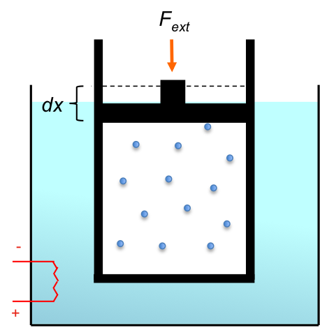
Consider a thermally-conducting, frictionless, piston-cylinder device immersed in a water bath whose temperature can be adjusted (see above diagram). The device is regarded as the system and contains a gas at an initial state of equilibrium A, which is characterised by thermodynamic properties like volume, pressure, temperature and entropy. The external pressure  is set equal to the pressure of the gas
  , and the bath, which is defined as the surroundings, has the same temperature as the device.
The change of state A to another equilibrium state B can be achieved through different paths or processes (see diagram below, which depicts the paths linking the two states of the system).

For example, we can successively reduce in infinitesimal steps at constant temperature such that each infinitesimal change is slow enough for the molecules to have sufficient time to equilibrate and spread evenly throughout the cylinder, resulting in uniform pressure and temperature throughout the system. This ensures that the thermodynamic properties of the system are well defined at every infinitesimal step and that we can determine and plot the change of values of these properties on a graph.
We can reverse the process from B to A by infinitesimally increasing , with the path taken being exactly the same as the forward process, except in the reverse direction. The infinitesimal increase or decrease in pressure implies that a reversible process requires infinite time to accomplish.
Another way to alter the state of the gas in the piston-cylinder device above is to instantaneously lower to the extent that the system only has enough time to equilibrate at the initial and final states but not at the intermediate states. We called such a path, an irreversible process.
As a reversible process is an idealised process, all real processes occurring within a finite timescale are considered irreversible. An irreversible path is shown as a dotted line on the graph, with only two points – the initial state and the final state – having defined properties and hence defined coordinates. The dotted line is drawn arbitrarily because there isn’t sufficient time for the system to equilibrate at the intermediate states, and hence no exact coordinates between A and B. Since the forward path of the irreversible process is poorly defined to begin with, we cannot explicitly describe the reverse path (other than another arbitrarily drawn dotted line) when we reverse the reaction irreversibly from B to A by instantaneously compressing the gas and transferring some heat from the system to its surroundings.
Although a reversible process is an idealised construct, it is used to derive most of the thermodynamic equations because equations require variables to be well defined to work.

Question
How do we apply thermodynamic equations that are derived from an idealised process to real processes?
Answer
A real process, when carried out slowly within a finite timeframe, approximates an ideal process. The graph below shows that the greater the number of well-defined intermediate points, the closer the real process is to an ideal one. Even if a real process cannot be carried out slowly, we can use thermodynamic equations to approximate results by making certain assumptions, e.g. uniform pressure and temperature of the system is maintained.

The concepts of reversibility and irreversibility are further elucidated in subsequent sections (see sections on entropy of an isolated system and Clausius inequality).
Question
Why is an irreversible process a spontaneous process?
Answer
This is due to the definition of a spontaneous process, which is defined as an irreversible process that occurs naturally under certain conditions in one direction, but requires continual external input in the reverse direction. See this article for details.
Lastly, reversible and irreversible processes can also be defined as follows:
A reversible process involves the passage of a system from its initial state to its final state and then back to the initial state without any change to either the system or the surroundings. However, the system and its surroundings cannot be simultaneously restored to their original states for an irreversible process.
In the above example involving the device in a water bath, both the system and the surroundings are precisely restored to their initial states for the reversible process (including no change in entropy of either the system and surroundings). As for the irreversible process, the system and its surroundings cannot be simultaneously restored to their initial states. If the system is restored to its initial state, a finite amount of heat must be transferred to the surroundings, leading to a positive change in entropy of the surroundings.
Question
What is the difference between a reversible reaction and a reversible process?
Answer
A reversible chemical reaction, e.g.  , is where X forms Y, and at the same time, Y forms X in a particular thermodynamic state. An irreversible reaction, denoted by
  , is when the reverse reaction cannot proceed in any state under reasonable conditions. On the other hand, a reversible process describes a path linking two thermodynamic states of a system, where thermodynamic properties of the system are well defined at all times.

For example, the above diagram shows four different states of the reaction , each with a set of well defined p, V and T. Since the reaction is reversible, X forms Y and Y forms X at any point on the graph. Let’s assume that the equilibrium amounts of X and Y at the four states are in the ratio of:
|
State
|
X:Y |
|
A
|
4:1
|
|
B
|
3:2
|
|
C
|
1:1
|
| D |
1:4
|
Clearly, there are different paths linking any two states. For example, if we want to convert an initial equilibrium amount of X and Y in the ratio 4:1 to a final equilibrium amount in the ratio of 1:1, we can accomplish that by infinitesimally increasing the volume of the system from  to
to  , followed by infinitesimally reducing of the pressure of the system from
  to
to  . Alternatively, we can proceed from A to D to C or directly from A to C.