In the previous article, we showed that the total  -component spin angular momentum operator
}) is
is }=\hat{S}_z^{\;&space;(1)}\otimes&space;I+I\otimes\hat{S}_z^{\;&space;(2)}) , which is a special case of the general form:
, which is a special case of the general form:
}\otimes&space;I+I\otimes\hat{M}_i^{\;&space;(2)}\;&space;\;&space;\;&space;\;&space;\;&space;\;&space;\;&space;\;&space;205)
 (where
  ) is the total angular momentum component operator.
 }) and
and }) are component operators of
are component operators of }) and
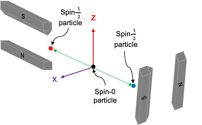
and }) respectively. and are operators of two sources of angular momentum. For example, they may be:
respectively. and are operators of two sources of angular momentum. For example, they may be:
1) the orbital angular momentum operator of particle 1 and orbital angular momentum operator of particle 2 respectively;
2) the spin angular momentum operator of particle 1 and spin angular momentum operator of particle 2 respectively;
3) the orbital angular momentum operator and spin angular momentum operator respectively of a particle;
4) the total angular momentum of particle 1 and the total angular momentum of particle 2.
Also mentioned in the previous article is that  and
and  . It is therefore easy to accept the validity of points 1) and 2). For point 3, the proposal that
  may seem untenable. However, spin angular momentum, like orbital angular momentum, is a form of angular momentum. In fact, the total angular momentum
  of a system is defined as the vector sum
  . If point 3) is valid, must satisfy the same commutation relations as described by eq99, eq100 and eq101.

Question
Show that satisfies the same commutation relations as described by eq99, eq100 and eq101.
Answer
![\left [ \hat{J}_x,\hat{J}_y \right ]=\left [\hat{M}_x^{\; (1)}\otimes I+I\otimes\hat{M}_x^{\; (2)},\hat{M}_y^{\; (1)}\otimes I+I\otimes\hat{M}_y^{\; (2)}\right ]](https://latex.codecogs.com/gif.latex?\left&space;[&space;\hat{J}_x,\hat{J}_y&space;\right&space;]=\left&space;[\hat{M}_x^{\;&space;(1)}\otimes&space;I+I\otimes\hat{M}_x^{\;&space;(2)},\hat{M}_y^{\;&space;(1)}\otimes&space;I+I\otimes\hat{M}_y^{\;&space;(2)}\right&space;])
Expanding the RHS of the above equation and noting that and commute because they act on different vector spaces, we have
![\left [ \hat{J}_x,\hat{J}_y \right ]=\left [\hat{M}_x^{\; (1)}\otimes I,\hat{M}_y^{\; (1)}\otimes I\right ] +\left [I\otimes\hat{M}_x^{\; (2)},I\otimes\hat{M}_y^{\; (2)}\right ]](https://latex.codecogs.com/gif.latex?\left&space;[&space;\hat{J}_x,\hat{J}_y&space;\right&space;]=\left&space;[\hat{M}_x^{\;&space;(1)}\otimes&space;I,\hat{M}_y^{\;&space;(1)}\otimes&space;I\right&space;]&space;+\left&space;[I\otimes\hat{M}_x^{\;&space;(2)},I\otimes\hat{M}_y^{\;&space;(2)}\right&space;])
![\left [ \hat{J}_x,\hat{J}_y \right ]=\left [\hat{M}_x^{\; (1)} ,\hat{M}_y^{\; (1)}\right ]\otimes I +I\otimes\left [\hat{M}_x^{\; (2)},\hat{M}_y^{\; (2)}\right ]](https://latex.codecogs.com/gif.latex?\left&space;[&space;\hat{J}_x,\hat{J}_y&space;\right&space;]=\left&space;[\hat{M}_x^{\;&space;(1)}&space;,\hat{M}_y^{\;&space;(1)}\right&space;]\otimes&space;I&space;+I\otimes\left&space;[\hat{M}_x^{\;&space;(2)},\hat{M}_y^{\;&space;(2)}\right&space;])
With reference to eq99, eq100, eq101, eq165, eq166 and eq167, ![\left [\hat{M}_i^{\; (l)} ,\hat{M}_j^{\; (l)}\right ]=i\hbar\epsilon_{ijk}\hat{M}_k^{\; l}](https://latex.codecogs.com/gif.latex?\left&space;[\hat{M}_i^{\;&space;(l)}&space;,\hat{M}_j^{\;&space;(l)}\right&space;]=i\hbar\epsilon_{ijk}\hat{M}_k^{\;&space;l}) , where
, where  and
and  is the Levi-Civita symbol. So,
![\left [ \hat{J}_x,\hat{J}_y \right ]=i\hbar\hat{M}_z^{\; (1)} \otimes I +i\hbar I\otimes\hat{M}_z^{\; (2)}=i\hbar\hat{J}_z](https://latex.codecogs.com/gif.latex?\left&space;[&space;\hat{J}_x,\hat{J}_y&space;\right&space;]=i\hbar\hat{M}_z^{\;&space;(1)}&space;\otimes&space;I&space;+i\hbar&space;I\otimes\hat{M}_z^{\;&space;(2)}=i\hbar\hat{J}_z)
Similarly, we have ![\left [ \hat{J}_y,\hat{J}_z \right ]=i\hbar\hat{J}_x](https://latex.codecogs.com/gif.latex?\left&space;[&space;\hat{J}_y,\hat{J}_z&space;\right&space;]=i\hbar\hat{J}_x) and
and ![\left [ \hat{J}_z,\hat{J}_x \right ]=i\hbar\hat{J}_y](https://latex.codecogs.com/gif.latex?\left&space;[&space;\hat{J}_z,\hat{J}_x&space;\right&space;]=i\hbar\hat{J}_y) .
.
Since the total angular momentum component operators satisfy the form of commutation relations as described by eq99, eq100 and eq101, the raising and lowering operators also apply to the total angular momentum operator  . We would therefore expect
\hbar^2\psi\;&space;\;&space;\;&space;\;&space;and\;&space;\;&space;\;&space;\;&space;\;&space;\hat{J}_z\psi=m_j\hbar\psi\;&space;\;&space;\;&space;\;&space;\;&space;\;&space;\;&space;\;&space;\;&space;205a)
You’ll realise from the workings of the above Q&A that we can simplify the notation  of eq205 as

To show that commutes with  , where can be either
  or
or  , we have
 ![\left [ \hat{J}_z,\hat{l}_z \right ]=\left [ \hat{l}_z,\hat{l}_z \right ]+\left [ \hat{s}_z,\hat{l}_z \right ]=0](https://latex.codecogs.com/gif.latex?\left&space;[&space;\hat{J}_z,\hat{l}_z&space;\right&space;]=\left&space;[&space;\hat{l}_z,\hat{l}_z&space;\right&space;]+\left&space;[&space;\hat{s}_z,\hat{l}_z&space;\right&space;]=0) and
and ![\left [ \hat{J}_z,\hat{s}_z \right ]=\left [ \hat{l}_z,\hat{s}_z \right ]+\left [ \hat{s}_z,\hat{s}_z \right ]=0](https://latex.codecogs.com/gif.latex?\left&space;[&space;\hat{J}_z,\hat{s}_z&space;\right&space;]=\left&space;[&space;\hat{l}_z,\hat{s}_z&space;\right&space;]+\left&space;[&space;\hat{s}_z,\hat{s}_z&space;\right&space;]=0) . Therefore, the eigenstate of is simultaneously the eigenstates of
. Therefore, the eigenstate of is simultaneously the eigenstates of  and
and  . This implies that the eigenvalues of are the sum of the eigenvalues of and , i.e.
  , or
, or

In other words, the allowed values of the total magnetic quantum number  are the sum of the allowed values of the two contributing magnetic quantum numbers. As for the allowed values of the total angular momentum quantum number
  , let’s further define the eigenvalues of
  and
and  as
as \hbar^{2}) and
and \hbar^{2}) respectively. This allows us to work with the quantum numbers
respectively. This allows us to work with the quantum numbers  and
and  .
.
Now, the maximum value of in eq207 is  . Since the maximum value of a magnetic quantum number is the angular momentum quantum number (i.e.
  and
and  , where
  ), the highest value of is

Furthermore, for a particular value of  in the coupled representation, there are
  values of and therefore states. So
  has
has  states. These states are
  . The states for the next lower value of (denoted by
  ) are
) are  . The same logic applies for states all the way to the lowest value of .
Question
Show that the total number of states in the uncoupled representation is (2M_2+1)) .
.
Answer
In eq193, the total number of states in the uncoupled representation  is the number of ways to form Kronecker products of basis vectors from each vector space. Since there are
  basis vectors in the 1st vector space and
  basis vectors in the 2nd vector space,
(2M_2+1)\;&space;\;&space;\;&space;\;&space;\;&space;\;&space;\;&space;\;&space;209)
To determine the lower values of , we consider the lower values of  , the first being
  . There are two possible ways to obtain this value, with
  and
and  , or
, or  and
and  . Since each state is characterised by a unique value of for a particular value of , one of the two possibilities is accounted for by the state
  . The remaining possibility must be due to
  . Since , we must have
  . Furthermore, because , we have
  . The state is therefore
  .
.
For  , there are three possible ways to obtain it. Again, one of the possible ways is accounted for by
  and the second way by
  . The remaining possibility must be due to the state
  .
.
Therefore, the allowed values of are

or

To determine  , we note that the total number of states for the system can be written as
 ) because there are states associated with each value of . Since
because there are states associated with each value of . Since  , we can further split the sum as:
-\sum_{j=0}^{j_{min}-1}(2j+1)\;&space;\;&space;\;&space;\;&space;\;&space;\;&space;\;&space;\;&space;210)
Question
Show that =n^{2}) and hence
and hence =(x+1)^{2}) .
.
Answer
=1+\sum_{j=1}^{n-1}(2j+1)=1+2\sum_{j=1}^{n-1}j+\sum_{j=1}^{n-1}1\;&space;\;&space;\;&space;\;&space;\;&space;\;&space;\;&space;\;&space;211)
For the 2nd term on RHS of 2nd equality of eq211, +(n-1)) , which if written in the reverse order becomes
, which if written in the reverse order becomes +(n-2)+\cdots+2+1) . Adding the two sums, we have
. Adding the two sums, we have
\;&space;\;&space;\;&space;\;&space;\;&space;\;&space;\;&space;\;&space;214)
For the 3rd term on RHS of 2nd equality of in eq211

Substitute eq214 and eq215 back in eq211, we have . Let  , we have
=(x+1)^{2}\;&space;\;&space;\;&space;\;&space;\;&space;\;&space;\;&space;\;&space;216)
Using eq216, where  for
for ) , and
, and  for
for ) , eq210 becomes
, eq210 becomes
^{2}-j_{min}^{\;&space;\;\;&space;\;&space;\;&space;\;&space;2}=j_{max}^{\;&space;\;\;&space;\;&space;\;&space;\;&space;2}+2j_{max}+1-j_{min}^{\;&space;\;\;&space;\;&space;\;&space;\;&space;2}\;&space;\;&space;\;&space;\;&space;\;&space;\;&space;\;&space;\;&space;217)
The total number of states (energy levels) of a system must be independent of the chosen representation. Substituting eq209 in LHS of eq217 and eq208 in RHS of eq217 and simplifying,
\;&space;\;&space;\;&space;\;&space;\;&space;\;&space;\;&space;\;&space;218)
Eq218 is equivalent to  because ,
  ,
,  , and may be a larger value than . Therefore, for a given value of and a given value of , the allowed values of the total angular momentum quantum number are:

which is called the Clebsch-Gordan series.
Question
Write all the eigenstates (in the form of  ) and basis states (in the form of
  ) of a system with two sources of angular momentum,
  and
and  .
.
Answer
There are a total of 15 eigenstates and also 15 basis states. The allowed values of are 3, 2 and 1. The eigenstates are  ,
,  ,
,  ,
,  ,
,  ,
,  ,
,  ,
,  ,
,  ,
,  ,
,  ,
,  ,
,  ,
,  and
and  . The basis states are , ,
  ,
,  ,
,  , , , , ,
  ,
,  ,
,  ,
,  ,
,  and
and  . Each spin eigenstate of the system is a linear combination of the 15 basis states.
What we have described so far pertains to a system with two sources of angular momentum. If the system has more than two sources of angular momentum, the Clebsch-Gordan series is applied repeatedly, i.e. a first series is written with and , and then the Clebsch-Gordan procedure is again applied to each value of this series with  to form a second resultant series, and the procedure is repeated until a final resultant series is developed with
  . For example, a system with three sources of angular momentum,
  ,
,  and
and  , has the following allowed values of
  :
:
1st series using  and
and  ,
, 
2nd and final series using  and
and  ,
, 
For this system, there are 8 basis states, whose explicit forms can be expressed as follows: