Perturbation theory is a method for finding an approximate solution to a problem by building on exact solutions of a simpler and related problem.
Consider the eigenvalue equation of
where is the non-relativistic Hamiltonian,
is a complete set of orthonormal eigenfunctions that spans a Hilbert space, and
represents the exact eigenvalue solutions. We call
and
the unperturbed Hamiltonian and unperturbed set of wavefunctions respectively.
If we extend the non-relativistic Hamiltonian to include certain interactions like spin-orbit coupling or a potential due to a ligand field, our eigenvalue equation in general is:
where and
are the perturbed Hamiltonian and perturbed set of wavefunctions respectively.
One common method of approximation is to write the new perturbed Hamiltonian as a power series in an arbitrary parameter :
where and
are the first-order and second-order corrections respectively to
.
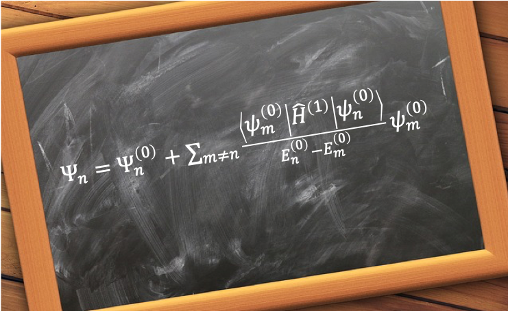
Similarly, the associated perturbed wavefunctions and energies of perturbed states are:
If we are satisfied with using just the first two terms in each of the power series of eq264, eq265 and eq266 for the approximation, we are dealing with what is known as the first-order perturbation theory. Substituting the first two terms in each of the three equations in eq263 and ignoring second-order quantities,
Since the parameters are arbitrary, they can be non-zero. If so, the only way to satisfy eq266 when is for
,
,
and so on to be zero. This implies that the powers of
are independent variables. Consequently, the coefficients in eq266a must be zero:
Substituting and
in eq267,
To find , we multiply eq268 by
and integrate; and use eq36 and the orthonormality of
,
Eq269 reveals that we can compute using the first-order Hamiltonian and the complete set of wavefunctions of
. However, the equation only works if all the wavefunctions are non-degenerate. To explain this limitation, we have to find the expression for
. Since
, the unperturbed wavefunction
can be fully characterised by the complete set
. We therefore expand
, which belongs to the same Hilbert space, as a linear combination of
.

Question
Show that writing the linear combination as (i.e.
has no
component) ensures that
in eq263 is normalised with respect to the first order of
.
Answer
When is normalised,
. Substituting eq265 in this equation and expanding up to
,
If has no
component, i.e.
,
Rearranging eq268 to and substituting
in the equation,
Multiplying the above equation by and integrating,
If , the above equation reduces to eq269. If
, only the term with
survives, giving:
Substituting the above equation in ,
The total wavefunction is . If
, we have a problem. So, eq269 only works when all the wavefunctions are non-degenerate. If some of the wavefunctions are degenerate, we require another method called degenerate perturbation theory to calculate the eigenvalues.
To derive the second-order energy correction, we consider the following Schrodinger equation:
where we have used just a first-order correction to the Hamiltonian to simplify the calculations.
Collecting the powers of and letting the coefficient be zero, we have
Multiplying the above equation by and integrating over all space,
Using eq35, . So,
For ,
Since , we have
. So,
It follows that the second-order energy depends on , which is a linear combination (mixing) of all other unperturbed eigenstates.
Substituting again and eq269a in the above equation, and using eq35 yields