Intermediate Chemistry - Mono Mole

September 16, 2019June 12, 2025

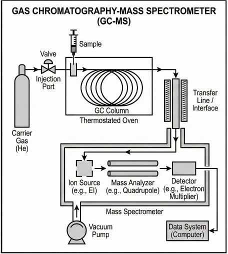
Mass spectrometry application: relative atomic mass

Mass spectrometry plays a crucial role in determining relative atomic mass by accurately measuring the masses of isotopes in a sample, providing essential data for understanding elemental abundance and chemical properties.

As mention in an earlier article, the relative masses of isotopes can be determined by comparing the charge-to-mass ratio of an isotope of interest with that of carbon-12. For example, mass spectrometric data for the ratio of the mass-to-charge ratio (u/z) of ²H to that of ¹²C is 0.167842. Thus, the relative mass of ²H on the carbon-12 unified atomic mass unit scale is:

$u\; of \; ^{2}H=\frac{u/z\; of\;\; ^2H}{u/z\; of\; \; ^{12}C}\; \times \; u\; of\; ^{12}C$

$u\; of \; ^{2}H=0.167842\times 12\, u$

$u\; of \; ^{2}H=2.014104\, u$

Consequently, the relative atomic mass of an element can be calculated from its isotopic abundance spectrum.

With reference to the spectrum above, the relative atomic mass of chlorine is:

$A_{r,Cl}=\frac{100\times 34.969}{100+31.96}+\frac{31.96\times 36.966}{100+31.96}=35.45$

Question

Deduce the spectrum for the chlorine gas ion, Cl₂⁺.

Isotope	Relative isotopic mass	Relative abundance, %
³⁵Cl	35	75.78
³⁷Cl	37	24.22

Answer

Assuming a random distribution of isotopes in the sample of chlorine gas and no fragmentation, the possible permutations of chlorine isotopes in a chlorine gas ion are:

Permutation, ^XCl^YCl⁺	Relative isotopic mass	No. of permutations
³⁵Cl³⁵Cl	70	1
³⁵Cl³⁷Cl or ³⁷Cl³⁵Cl	72	2
³⁷Cl³⁷Cl	74	1

The probability of observing each permutation is:

Permutation, ^XCl^YCl⁺	Probability = abundance X x abundance Y x no. of permutations
³⁵Cl³⁵Cl	0.7578 x 0.7578 x 1 = 0.5742
³⁵Cl³⁷Cl or ³⁷Cl³⁵Cl	0.7578 x 0.2422 x 2 = 0.3671
³⁷Cl³⁷Cl	0.2422 x 0.2422 x 1 = 0.0587

Hence, the spectrum has the following characteristics:

Permutation	Relative isotopic mass	Relative abundance (%)	% of predominant peak
³⁵Cl³⁵Cl	70	57.42	100.00
³⁵Cl³⁷Cl or ³⁷Cl³⁵Cl	72	36.71	63.93
³⁷Cl³⁷Cl	74	5.87	10.22

The values for ‘% of predominant peak’ are calculated relative to the abundance of ³⁵Cl³⁵Cl.

Here’s another way to explain the permutation of isotopes in chlorine gas:

Chlorine gas is formed by the collision of two chlorine atoms. Consider an infinitesimal two-dimensional space in a vessel that is filled with chlorine atoms, with the space large enough to accommodate two chlorine atoms (see diagram below).

If we further consider a single axis of collision through that space, and that chlorine atoms are approaching the space along that axis from the left and from the right, we end up with four possible products: ³⁵Cl³⁵Cl, ³⁵Cl³⁷Cl,³⁷Cl³⁵Cl and ³⁷Cl³⁷Cl. If the abundances of ³⁵Cl and ³⁷Cl are equal, we have twice as many chlorine molecules with mixed isotopes than ³⁵Cl³⁵Cl or ³⁷Cl³⁷Cl, i.e. in the ratio of 2:1:1. If the abundances of ³⁵Cl and ³⁷Cl are unequal, we multiply the numbers in the ratio with the respective abundances of isotopes to get the probabilities of occurrence of the three molecular species. The same result is obtained if we rotate the axis of collision in any direction in three dimensions, or if the collision happens at an angle.

next article: application: structure elucidation

Previous article: Modern mass spectrometer design

Content page of mass spectrometry

Content page of intermediate chemistry

Main content page

September 16, 2019November 17, 2024

Modern mass spectrometer design

The modern mass spectrometer, an advanced analytical instrument, precisely measures the mass-to-charge ratios of ions, enabling detailed analysis of molecular composition and structure across a wide range of scientific fields.

As mentioned in an earlier article, J. J. Thomson constructed one of the earliest mass spectrometers and conducted the well-known experiment to determine the mass-to-charge ratio of an electron. Since then, different mass spectrometer designs have been developed. For instance, a typical modern Thermal Ionisation Mass Spectrometer (TIMS) consists of the following:

- Ioniser, where the sample to be analysed is bombarded by electrons to form ions and ion fragments, which are then accelerated into the mass analyser.
- Mass analyser that utilises a magnetic field to deflect and separate the ions according to their mass-to-charge ratios (u/z). Note that the mass-to-charge ratios before the 1980s were quoted in u/e where e is the charge of an electron instead the number of charges, which is z.
- Detector that measures the abundance of ions with reference to their mass-to-charge ratios and converts the data into electrical signals.

The result is a plot of ion abundance versus mass-to-charge ratio, with the height of the peaks normalised to the most abundant ion in the spectrum.

next article: application: relative atomic mass

Previous article: application: relative isotopic mass

Content page of mass spectrometry

Content page of intermediate chemistry

Main content page

September 15, 2019September 25, 2024

How to select an appropriate pH indicator for titration?

How do we select an appropriate pH indicator for titration?

Let’s consider the same indicator as in the previous article: bromocresol green. If the pH of the analyte containing bromocresol green is between 0 and 3.8, it appears yellow; if the pH is between 5.4 and 14, it appears blue. Between 3.8 and 5.4, the colour changes from yellow to blue as the concentration ratio of [In^–]/[HIn] changes from 10 to 0.1. In fact, when [In^–] = [HIn], the colour of the titrand is green, indicating equal amounts of the yellow acid and the blue conjugate base.

Therefore, bromocresol green is a suitable indicator for a titration with a stoichiometric point (SP) that involves a sharp change of pH from less than 3.8 to more than 5.4 when about 0.1 cm³ of solution (about two drops) is added to the analyte. For example, the titration of 10 cm³ of 0.200 M of HCl with 0.100 M of NaOH sees a colour change of yellow to blue at the SP (see table and graph below).

	One drop before SP	SP	One drop after SP
Volume, cm³	19.95	20.00	20.05
pH	3.78	7.00	10.22

In other words, a suitable pH indicator for titration is one whose pH range is narrower than and within the range of the change in pH of the analyte at the stoichiometric point (ideally with one or two drops of solution added).

Another example is the titration of 10 cm³ of 0.200 M of aqueous NH₃ (K_a = 1.8 x 10^-5) with 0.100 M of HCl, which sees a colour change from blue to yellow at the SP (see table and graph below).

	One drop before SP	SP	One drop after SP
Volume, cm³	19.95	20.00	20.05
pH	6.65	5.22	3.78

The following table lists some common indicators and their pH ranges:

Indicator	Low pH colour	pH range	High pH colour	pK_a
Thymol blue (first transition)	red	1.2 – 2.8	yellow	1.65
Thymol blue (second transition)	yellow	8.0 – 9.6	blue	8.96
Methyl yellow	red	2.9 – 4.0	yellow	3.30
Bromophenol blue	yellow	3.0 – 4.6	blue	3.85
Congo red	blue-violet	3.0 – 5.0	red	4.10
Methyl orange	red	3.1 – 4.4	yellow	3.46
Screened methyl orange (second transition)	purple-grey	3.2 – 4.2	green	3.70
Bromocresol green	yellow	3.8 – 5.4	blue	4.66
Methyl red	red	4.4 – 6.2	yellow	5.00
Bromothymol blue (second transition)	yellow	6.0 – 7.6	blue	7.10
Phenol red	yellow	6.4 – 8.0	red	7.81
Phenolphthalein (second transition)	colorless	8.3 – 10.0	purple-pink	9.30
Thymolphthalein (second transition)	colorless	9.3 – 10.5	blue	9.90
Alizarine Yellow R	yellow	10.2 – 12.0	red	11.2
Indigo carmine	blue	11.4 – 13.0	yellow	12.2

Next article: structures of common indicators

PREVIOUS ARTICLE: THE PH RANGE OF AN INDICATOR

Content page of ph indicators

Content page of Intermediate chemistry

Main content page

September 15, 2019May 6, 2025

Structures of common indicators

The diverse chemical structures of common pH indicators, ranging from simple organic dyes to complex conjugated systems, play a crucial role in their ability to visually signal changes in acidity and alkalinity.

Methyl orange is a commonly used indicator. At low pH, protonation of the nitrogen at the para position of the benzenesulphonate moiety is preferred over protonation of the negatively charged oxygen in the sulphonate group, as this confers resonance stabilization (benzenoid-quinonoid tautomerism) to the acid form of methyl orange.

Litmus, extracted from lichen, is processed and applied onto filter paper. It has a pH range of 4.5 to 8.3 and contains the chromophore, 7-hydroxyphenoxazone, which occurs in the following states:

Phenolphthalein has three pK_a values with four different forms. However, stoichiometric points of titrations are most commonly monitored with the middle pK_a value of 9.30, which involves the lactone and phenolate (dianionic) forms:

Thymol blue has two transition range with pKa₁ = 1.65 and pKa₂ = 8.96.

Diphenylamine acts as a redox indicator in titrations involving potassium dichromate (K₂Cr₂O₇). In a typical redox titration (e.g. FeSO₄ with K₂Cr₂O₇), once all Fe²⁺ is converted to Fe³⁺, any excess dichromate will begin to oxidise diphenylamine, which changes colour — typically from colourless to a deep blue or violet, indicating that the endpoint has been reached.

Previous article: How to select an appropriate ph indicator for titration?

Content page of ph indicators

Content page of Intermediate chemistry

Main content page

September 15, 2019May 6, 2025

The pH range of an indicator

The pH range of an indicator is the pH interval in which the indicator changes colour.

To elaborate further, we will use the Henderson-Hasselbalch equation to study the equilibrium of a pH indicator, which is a weak acid.

$pH=pK_{In}+log\frac{In^-}{HIn}$

Consider a titration using two drops of bromocresol green with pK_in= 4.7. We have

$pH=4.7+log\frac{In^-}{HIn}\; \; \; \; \; \; \; \; (1)$

Since the concentration of the indicator in the analyte is very low, the contribution of H⁺ from the indicator is negligible and does not affect the total concentration of H⁺ in the solution. Hence, the pH value in eq1 is solely due to the H⁺of the analyte; that is, the pH of the analyte determines the position of the equilibrium of the indicator.

When bromocresol green is predominantly in the form HIn, it appears yellow. If it is predominantly in the form In^–, we see it as blue.

$\begin{matrix} HIn(aq)\\yellow \end{matrix}\rightleftharpoons H^+(aq)+\begin{matrix} In^-(aq)\\blue \end{matrix}$

As a rule of thumb, our eyes can perceive a complete change in the colour of the indicator from its acid form to the conjugate base and vice versa, when the concentration of one form is ten times greater than the other. So, bromocresol green appears blue when:

$[In^-]\geqslant 10[HIn]\; \; \; \; \; \; \; \; (2)$

which corresponds to the indicator in a pH environment of pH ≥ 5.7 (by substituting eq2 in eq1).

At the other limit, bromocresol green appears yellow when:

$[HIn]\geqslant 10[In^-]\; \; \; \; \; \; \; \; (3)$

which corresponds to the indicator in a pH environment of pH ≤ 3.7 (by substituting eq3 in eq1).

In other words, if a few drops of bromocresol green are added to an analyte with a pH ≥ 5.7 and another with a pH ≤ 3.7, the solutions will appear blue and yellow, respectively.

We call this difference in pH (3.7 to 5.7 for bromocresol green) the pH range of the indicator.

NEXT ARTICLE: HOW TO SELECT an APPROPRIATE PH INDICATOR FOR TITRATION

Previous article: Overview

Content page of ph indicators

Content page of Intermediate chemistry

Main content page

September 15, 2019November 3, 2025

Strong base to weak acid titration curve: overview

We have explained the shape of a strong-base-to-strong-acid titration curve in a basic level article. We shall now describe the shape of a strong-base-to-weak-acid titration curve using simple equations like the Henderson-Hasselbalch equation. To do so, we need to analyse the curve at different stages of the titration. These stages are:

- Start point
- After start point but before stoichiometric point
- Maximum buffer capacity point
- Stoichiometric point
- Beyond stoichiometric point

Proceed to the next few articles to understand the mathematics and assumptions behind the formulae for the various stages of the pH curve.

next article: start point of titration

Content page of strong base to weak acid titration curve

Content page of intermediate chemistry

Main content page

September 15, 2019March 6, 2026

Stoichiometric point of titration

The stoichiometric point of titration is the moment when the moles of titrant added precisely neutralise the moles of analyte in the solution, indicating a complete reaction between the two species.

Generally, the pH of the titration of a strong acid and a strong base at the stoichiometric point is 7 at 25°C. However, the pH of the titration of a strong base and a weak acid at the stoichiometric point is greater than 7 at 25°C. This is because the salt of a weak acid and a strong base (e.g. CH₃COOH and NaOH) is a weak conjugate base, which hydrolyses in water, i.e. it reacts with water to reform the acid according to the following reaction:

$CH_3COO^-(aq)+H_2O(l)\; \begin{matrix}K_h\\ \rightleftharpoons \end{matrix}\; CH_3COOH(aq)+OH^-(aq)$

where K_his the hydrolysis constant.

This results in a basic solution since OH^– is formed. During the titration of a strong base and a weak acid between the start point and the stoichiometric point, the presence of unneutralised acid in the reaction flask causes the equilibrium of the hydrolysis reaction to shift to the left. However, when the stoichiometric point is reached, the weak acid is completely neutralised by the base and we can no longer ignore the effects of hydrolysis on the pH of the solution. Since,

$K_a=\frac{[CH_3COO^-][H^+]}{[CH_3COOH]}\; \; \; and\; \; \; K_w=[H^+][OH^-]$

$K_h=\frac{[CH_3COOH][OH^-]}{[CH_3COO^-]}=\frac{K_w}{K_a}$

From the hydrolysis equation, [CH₃COOH] = [OH^–], so

$\frac{K_w}{K_a}=\frac{[CH_3COOH][OH^-]}{[CH_3COO^-]}=\frac{[OH^-]^2}{[CH_3COO^-]}$

$[OH^-]=\sqrt{\frac{K_w}{K_a}[CH_3COO^-]}$

$\frac{K_w}{[H^+]}=\sqrt{\frac{K_w}{K_a}[CH_3COO^-]}$

Taking the logarithm on both sides of the above equation and applying the definitions of pH, pK_aand pK_w,

$pH=\frac{pK_w+pK_a+log[A^-]}{2}\; \; \; \; \; \; \; \; (4)$

where [A^–] = [CH₃COO^–], the concentration of the salt at the stoichiometric point before hydrolysis.

Eq4 is the general equation to calculate the pH of a strong base to weak acid titration at the stoichiometric point.

Question

Calculate the pH of the titration of 10 cm³ of 0.200 M of CH₃COOH (K_a = 1.75 x 10^-5) with 0.100 M of NaOH at the stoichiometric point.

Answer

Using eq4,

$pH=\frac{-log10^{-14}-log\left ( 1.75\times 10^{-5}\right)+log\left ( \frac{0.100\times 0.02}{0.01+0.02} \right )}{2}=8.79$

Note that [A^–] can be computed using either the acid or the base.

The same logic applies when determining the equation for the pH of a strong acid to weak base titration at the stoichiometric point, with the expected pH lower than 7.

Question

Calculate the pH of the titration of 25.0 cm³ of 0.200 M of aqueous ammonia (K_b = 1.8 x 10^-5) with 0.100 M of HCl at the stoichiometric point.

Answer

The salt NH₄Cl at the stoichiometric point undergoes the following hydrolysis:

$NH_4^+(aq)+H_2O(l)\; \begin{matrix}K_h\\ \rightleftharpoons \end{matrix}\; NH_4OH(aq)+H^+(aq)$

where $K_h=\frac{[NH_4OH][H^+]}{[NH_4^+]}=\frac{[H^+]^2}{[NH_4^+]}$ .

Since $K_b=\frac{[NH_4^+][OH^-]}{[NH_4OH]}$ and $K_w=[H^+][OH^-]$ , we have

$K_h=\frac{K_w}{K_b}=\frac{1.0\times 10^{-14}}{1.8\times 10^{-5}}=5.56\times 10^{-10}$

It follows that

$pH=-log\biggr\[\sqrt{\biggr$5.56\times 10^{-10}\times \frac{0.025\times 0.200}{0.025+0.050}\biggr$}\biggr\]=5.22$

next article: Beyond stoichiometric point of titration

Previous article: After start point and before stoichiometric point of titration

Content page of strong base to weak acid titration curve

Content page of intermediate chemistry

Main content page

September 15, 2019April 11, 2025

Beyond stoichiometric point of titration

Beyond the stoichiometric point of titration, the pH of the solution experiences significant shifts, often leading to rapid changes that highlight the excess of titrant and the resultant dominance of the strong base or acid in the solution.

To characterised this region, we make the following assumption:

- [OH^–] from water is negligible, i.e. pH of the solution is solely determined by [OH^–]_ex from the excess base added after the stoichiometric point, as the dissociation of water is again suppressed at this stage.

Even though the auto-dissociation of water is suppressed, water is still equilibrating between its molecular form and its ionic components. Applying the above assumption, the equilibrium constant of water is:

$K_w=[H^+][OH^-]\approx [H^+][OH^-]_{ex}$

Taking the logarithm on both sides of the above equation and applying the definitions of pH and pK_w,

$pH=pK_w+log[OH^-]_{ex}\; \; \; \; \; \; \; \; (5)$

Eq5 is the general equation to calculate the pH of a strong base to weak acid titration beyond its stoichiometric point. The same logic applies when determining the equation for the pH of a strong acid to weak base titration beyond the stoichiometric point.

The diagram below shows the superimposition of eq5 (purple curve) over the complete pH titration curve (blue curve), which disregards the above assumption, for the titration of 10 cm³ of 0.200 M of CH₃COOH (K_a = 1.75 x 10^-5) with 0.100 M of NaOH.

Even though the two curves appear to fit perfectly, they do not actually coalesce and are still two separate curves (discernible when the axes of the plot are scaled to a very high resolution). However, for practical purposes, eq5 is a very good approximation of a pH curve for the region beyond the stoichiometric point of a strong acid to weak base titration.

next article: Combining all equations

Previous article: stoichiometric point of titration

Content page of strong base to weak acid titration curve

Content page of intermediate chemistry

Main content page

September 15, 2019April 11, 2025

Start point of titration

The start point of a titration marks the initial pH of the solution before any titrant is added, serving as a crucial reference for analysing the subsequent changes in acidity or alkalinity throughout the process.

To characterised the start point, we begin with the following assumptions:

- [H⁺] from water is negligible, i.e. H⁺ in the flask containing the weak acid is solely due to that of the acid, [H⁺]_a, as the dissociation of water is suppressed at this stage.
- For a weak acid, [HA] is approximately equal to the concentration of the undissociated acid, [HA]_ud, i.e. the dissociation of the weak acid HA is negligible.

The equation for the dissociation of a weak monoprotic acid is:

$HA(aq)\rightleftharpoons H^+(aq)+A^-(aq)$

with the equilibrium constant at the start of the titration being:

$K_a=\frac{[H^+][A^-]}{[HA]}\approx \frac{[H^+]_a[A^-]}{[HA]_{ud}}=\frac{[H^+]_a\, ^2}{[HA]_{ud}}$

Taking the logarithm on both sides of the above equation and rearranging, we have:

$pH=\frac{pK_a-log[HA]_{ud}}{2}\; \; \; \; \; \; \; \; (1)$

Eq1 is the general formula for determining the pH of a strong base to weak acid titration at the start point.

The second assumption becomes less valid when the weak monoprotic acid or weak monoprotic base has K_a≥ 10^-3 or K_b≥ 10^-3respectively. Removing the second assumption, the equilibrium constant expression becomes:

$K_a\approx \frac{[H^+]_a[A^-]}{[HA]_{ud}-[H^+]_a}=\frac{[H^+]_a\, ^2}{[HA]_{ud}-[H^+]_a}$

The corresponding pH equation is obtained by rearranging the above equation into a quadratic equation in terms of [H⁺]_a, finding the latter’s roots and taking the logarithm of the root:

$pH=-log\left ( \frac{\sqrt{K_a\, ^2+4K_a[HA]_{ud}}-K_a}{2} \right )$

Question

Do both of the pH equations give the same pH value for the titration of 10 cm³ of 0.200 M of CH₃COOH (K_a = 1.75 x 10^-5) with NaOH?

Answer

Yes, both formulae give pH = 2.73. This validates the applicability of eq1 for acids with K_a in the region of 10^-5.

If we disregard both assumptions, we will end up deriving the complete pH titration curve for a strong base to weak acid titration. See this article in the advanced section for details.

Question

Show that pK_a + pK_b= 14.

Answer

$HA(aq)+H_2O(l)\rightleftharpoons H_3O^+(aq)+A^-(aq)$

$A^-(aq)+H_2O(l)\rightleftharpoons HA(aq)+OH^-(aq)$

$K_a=\frac{[H_3O^+][A^-]}{[HA]}\; \; \; \; \; \; \; \; K_b=\frac{[HA][OH^-]}{[A^-]}$

$-logK_a-logK_b=-log\frac{[H_3O^+][A^-]}{[HA]}-log\frac{[HA][OH^-]}{[A^-]}$

$pK_a+pK_b=-log[H_3O^+][OH^-]=pK_w=14$

next article: After start point and before stoichiometric point of titration

Previous article: overview

Content page of strong base to weak acid titration curve

Content page of intermediate chemistry

Main content page

September 15, 2019November 3, 2025

Strong base to weak acid titration curve: combining all equations

Equations describing the various stages of a titration provide a mathematical framework to quantify changes in pH of a solution, effectively illustrating the transition from the start point to the endpoint of the titration.

In summary, the pH curve of a strong base to weak acid titration can be described by the following simplified equations in place of a complex complete pH titration equation:

Start point	$pH=\frac{pK_a-log[HA]_{ud}}{2}\; \; \; \; \; \; \; \; (1)$
After start point but before stoichiometric point	$pH=pK_a+log\frac{[A^-]_s}{[HA]_r}\; \; \; \; \; \; \; \; (2)$
Maximum buffer capacity point	$pH=pK_a\; \; \; \; \; \; \; \; (3)$
Stoichiometric point	$pH=\frac{pK_w+pK_a+log[A^-]}{2}\; \; \; \; \; \; \; \; (4)$
Beyond stoichiometric point	$pH=pK_w+log[OH^-]_{ex}\; \; \; \; \; \; \; \; (5)$

The diagram below shows the plot of the above equations on a single graph for the titration of 10 cm³ of 0.200 M of CH₃COOH (K_a = 1.75 x 10^-5) with 0.100 M of NaOH:

A complementary set of equations can be derived using the same logic mentioned in the earlier articles to describe a strong acid to weak base titration.

Question

Answer

next article: application: structure elucidation

Previous article: Modern mass spectrometer design

next article: application: relative atomic mass

Previous article: application: relative isotopic mass

Next article: structures of common indicators

PREVIOUS ARTICLE: THE PH RANGE OF AN INDICATOR

Previous article: How to select an appropriate ph indicator for titration?

NEXT ARTICLE: HOW TO SELECT an APPROPRIATE PH INDICATOR FOR TITRATION

Previous article: Overview

next article: start point of titration

Question

Answer

Question

Answer

next article: Beyond stoichiometric point of titration

Previous article: After start point and before stoichiometric point of titration

next article: Combining all equations

Previous article: stoichiometric point of titration

Question

Answer

Question

Answer

next article: After start point and before stoichiometric point of titration

Previous article: overview

next article: Improved Henderson-Hasselbalch equation

Previous article: Beyond stoichiometric point of titration