The Coriolis effect is the apparent deflection of a moving object when observed from a rotating reference frame.
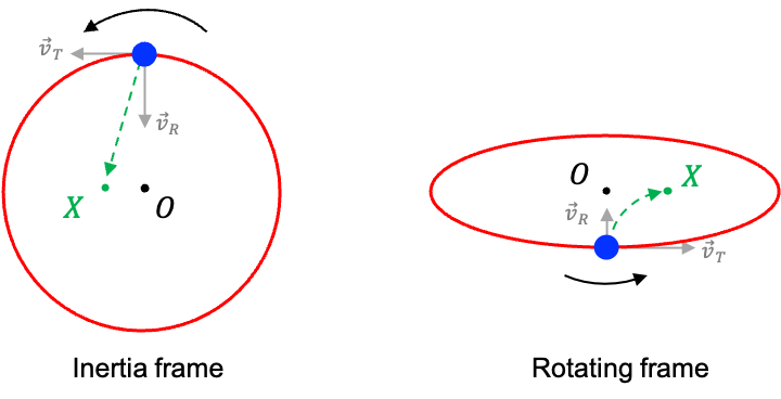
Consider a person holding a ball and standing on the edge of a large circular platform that is rotating anti-clockwise as viewed from above. At the twelve o’clock position, the person throws the ball directly towards the centre point O of the platform.
From the perspective of a stationary observer hovering above the platform (i.e. in an inertia frame of reference), the ball follows a straight-line path towards point X, slightly to the left of O. This trajectory occurs because, at the moment of release, the ball has two components of velocity:
-
- A radial component directed towards O.
- A tangential velocity due to the rotation of the platform at the point of release (in this case, towards the nine o’clock direction).
The resulting trajectory is the vector sum of these two components, which points towards X.
However, to the thrower, who is in the rotating frame of reference, the motion of the ball appears quite different. In this rotating frame, the ball seems to curve clockwise, as if being deflected to the right of its intended path. This illusion arises because, after release, the ball retains its original tangential speed, while the platform between the thrower and point O are rotating more slowly closer to the center, where tangential speed is lower. In other words, the ball appears to be moving ahead of the rotating platform beneath it.
It follows that an apparent force, acting perpendicular to the direction of the ball’s motion, is influencing its path. This fictitious force, introduced to account for the apparent deflection experienced in rotating frames, is known as the Coriolis force.
This phenomenon isn’t just a curiosity of rotating platforms. On the molecular level, the Coriolis force introduces a crucial vibration-rotation interaction (also known as Coriolis coupling) in the dynamics of a rotating molecule — an interaction that would otherwise be neglected in a first-order approximation, where vibration and rotation are treated as independent motions.
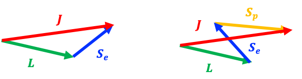
When a molecule rotates, its internal motion (vibration) occurs simultaneously within the rotating molecular frame. To an observer in this rotating frame, the atoms undergoing vibration appear to be deflected perpendicular to their vibrational velocity. The resulting Coriolis force, associated with this apparent deflection, acts to couple the molecule’s vibrational angular momentum with its overall rotational angular momentum.
In quantum mechanics, this coupling appears as an additional term in the Hamiltonian that couples vibrational and rotational states:
where is proportional to the product of vibrational and rotational angular momentum operators.
Explicitly,
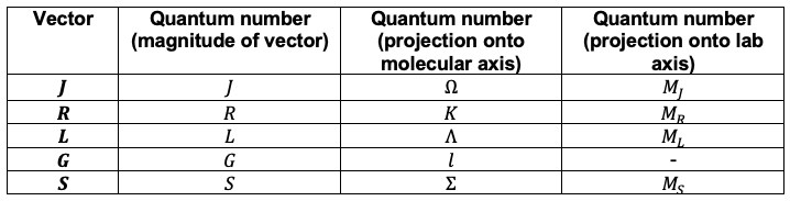
where
denotes the molecular principal axes (
).
is the operator for the
-component of the total angular momentum of the molecule (rotation).
is the operator for the
-component of the vibrational angular momentum.
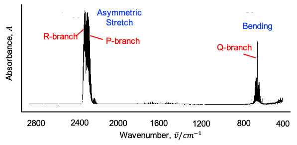
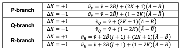
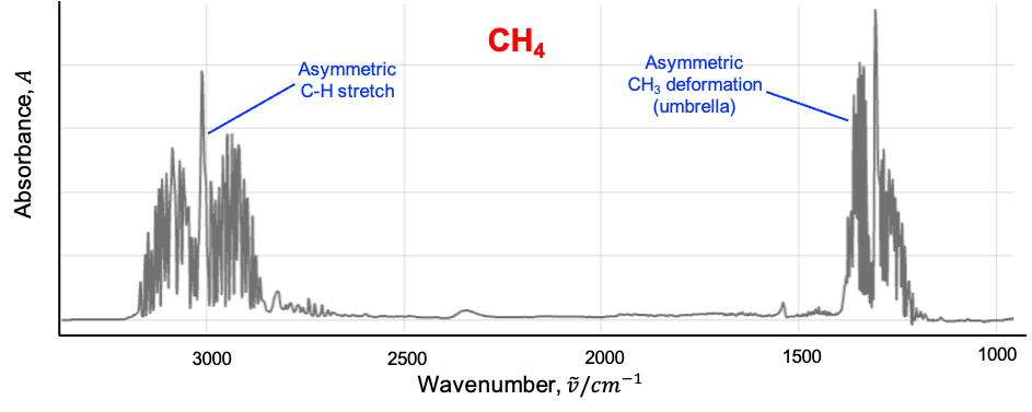
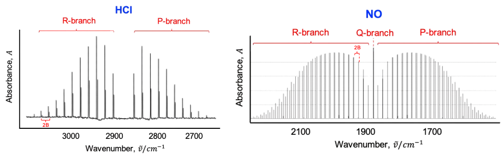
This leads to shifts in rotational energy levels depending on the vibrational state, as well as the splitting or mixing of rotational levels associated with degenerate vibrations. In the infrared spectrum, this manifests as an anomalous splitting of the P, Q and R branches.
On a much larger scale, the Coriolis effect plays a crucial role in shaping natural systems on Earth. Because Earth is a rotating sphere, this effect influences the motion of air masses, ocean currents and weather patterns. For instance, a cyclone’s spin results from two forces acting on the atmosphere simultaneously:
-
- The pressure gradient force moves air from a high-pressure region to a low-pressure region.
- The Coriolis effect deflects that moving air
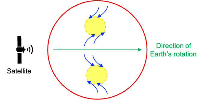
A low-pressure system is essentially a partial vacuum that draws in air from all directions. Consider a low-pressure region in the Northern Hemisphere (the upper yellow region in the diagram below). To an observer in a rotating frame of reference (e.g. a satellite moving at the same angular velocity as Earth from west to east), winds moving from the equator towards the low-pressure region appear to be deflected to the right, while winds flowing towards the region from the north appear to be deflected to the left. The combined movements result in an anti-clockwise sprial. The same principle causes winds to sprial clockwise in the Southern Hemisphere.
In conclusion, the Coriolis effect demonstrates the profound influence of rotational motion across vastly different scales — from affecting molecular behaviour to shaping global weather systems. At the molecular level, the principle manifests as Coriolis coupling, where rotational motion interacts with vibrational motion, subtly altering energy levels and spectral properties. On Earth, it governs the deflection of winds and ocean currents, giving rise to the rotation of cyclones and other large-scale atmospheric patterns. Together, these phenomena highlight the unifying power of rotational dynamics in both macroscopic and microscopic systems.