How can we mathematically describe the titration curve of a weak monoprotic acid versus a strong monoprotic base, after the start point and before the stoichiometric point?
To do so, we will make the following assumptions:
-
- [H+] from water is negligible, i.e. H+ in the flask containing the weak acid comes solely from the acid, [H+]a, as water dissociation is suppressed at this stage. This is because Ka ≫ Kw, which shifts the equilibrium H2O ⇌ H+ + OH– to the left.
- For a weak acid, [HA] is approximately equal to the concentration of the undissociated acid, [HA]ud, i.e. the weak acid HA dissociates only slightly, with the remaining concentration of HA after the addition of base approximated as [HA]r = [HA]ud – [A–]s, where [A–]s is concentration of the salt formed. This implies that:
- [A–] is approximately equal to the concentration of the salt, [A–]s, in the solution. In other words, A– is completely attributed to the salt formed, with no contribution from the further dissociation of HA.
- Hydrolysis of the salt is suppressed at this stage of the titration due to the overwhelming presence of HA, which shifts the hydrolysis equilibrium A–+ H2O ⇌ HA + OH– to the left.

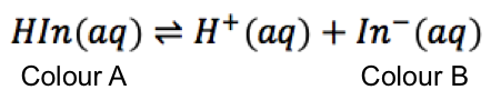
The equation for the dissociation of a weak monoprotic acid is
\rightleftharpoons&space;H^+(aq)+A^-(aq))
Using the assumptions, the equilibrium constant after start point and before stoichiometric point is:
![K_a=\frac{[H^+]_a[A^-]_s}{[HA]_r}](https://latex.codecogs.com/gif.latex?K_a=\frac{[H^+]_a[A^-]_s}{[HA]_r})
Taking the logarithm on both sides and apply the definitions of pH and pKa,
![pH=pK_a+log\frac{[A^-]_s}{[HA]_r}\; \; \; \; \; \; \; \; (2)](https://latex.codecogs.com/gif.latex?pH=pK_a+log\frac{[A^-]_s}{[HA]_r}\;&space;\;&space;\;&space;\;&space;\;&space;\;&space;\;&space;\;&space;(2))
Eq2 is known as the Henderson-Hasselbalch equation, which is a good approximation of the pH curve after the start point and before the stoichiometric point for a strong base to weak acid titration with Ka ≤ 10-3 (or a strong acid to weak base titration with Kb ≤ 10-3).

Question
Rewrite eq2 to include the volume of acid Va and the volume of base Vb.
Answer
![pH=pK_a+log\left ( \frac{[B]V_b}{V_a+V_b}/\frac{[A]V_a-[B]V_b}{V_a+V_b} \right )](https://latex.codecogs.com/gif.latex?pH=pK_a+log\left&space;(&space;\frac{[B]V_b}{V_a+V_b}/\frac{[A]V_a-[B]V_b}{V_a+V_b}&space;\right&space;))
![pH=pK_a+log\left ( \frac{[B]V_b}{[A]V_a-[B]V_b} \right )\; \; \; \; \; \; \; \; (2a)](https://latex.codecogs.com/gif.latex?pH=pK_a+log\left&space;(&space;\frac{[B]V_b}{[A]V_a-[B]V_b}&space;\right&space;)\;&space;\;&space;\;&space;\;&space;\;&space;\;&space;\;&space;\;&space;(2a))
where [A] = [HA]ud , and [B] is the initial concentration of the monoprotic base.
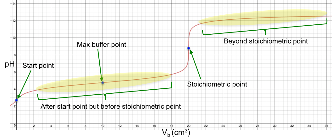
When eq2a is plotted as pH versus Vb, a titration curve is obtained (see diagram below).
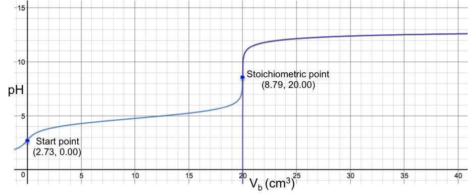
The diagram below is the superimposition of a green curve (the Henderson-Hasselbalch equation, eq2a) on a blue curve (the complete pH titration curve, which disregards all assumptions above), for the titration of 10 cm3 of 0.200 M of CH3COOH (Ka = 1.75 x 10⁻⁵) with 0.100 M of NaOH.
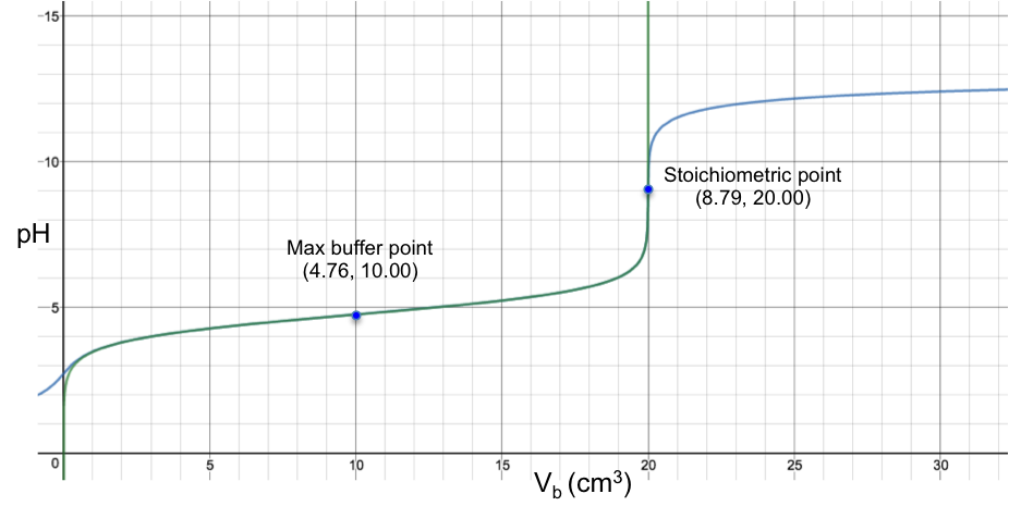
Even though the two curves appear to fit perfectly (apart from the initial bit before 1.00 cm3 and after the stoichiometric point), they do not actually coalesce and are still two separate curves (discernible when the axes of the plot are scaled to a very high resolution). However, for practical purposes, the Henderson-Hasselbalch equation is a very good approximation of a pH curve for the region after the start point and before the stoichiometric point for a strong base to weak acid titration.
When [A–]s = [HA]r , eq2 becomes
)
Eq3 occurs when the amount of salt formed equals to [HA]ud/2, i.e. when half of the acid is neutralised. This stoichiometric relation corresponds to the curve’s inflexion point, which is also called the maximum buffer capacity point.
Question
Why does the solution have maximum buffer capacity when half of the acid is neutralised, i.e. at the half-way volume point between the start point and the stoichiometric point?
Answer
For the buffer to be most effective, it has to resist to the greatest extent the change in pH versus the change in volume of base added. This means that the maximum buffer capacity corresponds to the point where the gradient of the function of eq2a is a minimum, i.e. at the inflexion point (see above diagram).
Taking the 2nd derivative of eq2a with respect to Vb and letting  gives
gives

where ![n_b=\left [ B \right ]V_b](https://latex.codecogs.com/gif.latex?n_b=\left&space;[&space;B&space;\right&space;]V_b) and
and ![n_a=\left [ A \right ]V_a](https://latex.codecogs.com/gif.latex?n_a=\left&space;[&space;A&space;\right&space;]V_a) .
.
Therefore, the inflection point occurs when the moles of added base equal half the moles of the undissociated acid, corresponding to half the total volume of base required for complete neutralisation.
If you want a full mathematical description of the maximum buffer capacity of a weak acidic buffer, read this article in the advanced section.
For a strong acid to weak base titration, we have the following weak base equilibrium:
\rightleftharpoons&space;B^+(aq)+OH^-(aq))
![K_b=\frac{[B^+][OH^-]}{[BOH]}](https://latex.codecogs.com/gif.latex?K_b=\frac{[B^+][OH^-]}{[BOH]})
Taking the logarithm on both sides of the above equation and rearranging,
![pOH=pK_b+log\frac{[B^+]}{[BOH]}\; \; \; \; \; \; \; \; (3a)](https://latex.codecogs.com/gif.latex?pOH=pK_b+log\frac{[B^+]}{[BOH]}\;&space;\;&space;\;&space;\;&space;\;&space;\;&space;\;&space;\;&space;(3a))
Eq3a is the basic form of the Henderson-Hasselbalch equation.
With reference to eq2 (or eq3a), the pKa (or pKb) of the weak acid (or weak base) can be determined from the pH of a strong base to weak acid titration (or knowing the pOH of a strong acid to weak base titration) at the half-way volume point, where the logarithmic term becomes zero.
Question
Show that pKa + pKb = 14.
Answer
+H_2O(l)\rightleftharpoons&space;A^-(aq)+H_3O^+(aq))
+H_2O(l)\rightleftharpoons&space;HA(aq)+OH^-(aq))
![K_a=\frac{[A^-][H_3O^+]}{[HA]}\; \; \; \; \; \; \; \; K_b=\frac{[HA][OH^-]}{[A^-]}](https://latex.codecogs.com/gif.latex?K_a=\frac{[A^-][H_3O^+]}{[HA]}\;&space;\;&space;\;&space;\;&space;\;&space;\;&space;\;&space;\;&space;K_b=\frac{[HA][OH^-]}{[A^-]})
![pK_a+pK_b=-log\frac{[A^-][H_3O^+]}{[HA]}-log\frac{[HA][OH^-]}{[A^-]}](https://latex.codecogs.com/gif.latex?pK_a+pK_b=-log\frac{[A^-][H_3O^+]}{[HA]}-log\frac{[HA][OH^-]}{[A^-]})
![=-log[H_3O^+][OH^-]=-logK_w=14](https://latex.codecogs.com/gif.latex?=-log[H_3O^+][OH^-]=-logK_w=14)