Time-dependent perturbation theory

The time-dependent perturbation theory is a method for finding an approximate solution to a problem that is characterised by the time-varying properties of a quantum mechanical system. For example, the electronic state of a molecule exposed to electromagnetic radiation is constantly perturbed by the oscillating electromagnetic field. Time-dependent perturbation theory is key to finding solutions to such problems, and is used to calculate transition probabilities in spectroscopy.

Consider the unperturbed eigenvalue equation $\hat{H}^{(0)}\psi_k^{(0)}=E_k^{(0)}\psi_k^{(0)}$ given by eq262, where $\hat{H}^{(0)}$ is the unperturbed Hamiltonian, $\psi_k^{(0)}$ is a complete set of orthonormal eigenfunctions of $\hat{H}^{(0)}$ in a Hilbert space, and $E_k^{(0)}$ represents the exact eigenvalue solutions. Furthermore, let’s rewrite eq57

$i\hbar\frac{\partial\Psi}{\partial t}=\hat{H}^{(0)}\Psi\;\;\;\;\;\;\;\;281a$

where $\hat{H}^{(0)}=-\frac{\hbar^2}{2m}\frac{\partial^2}{\partial x^2}+V$

$\Psi$ is the solution of the time-dependent Schrodinger equation. If it describes a stationary state, then

$\Psi=\psi_n^{(0)}e^{-i\frac{E_n^{(0)}t}{\hbar}}\;\;\;\;\;\;\;\;281b$

Otherwise, $\Psi$ can be expressed generally as the linear combination $\Psi=\sum_kc_k\psi_k^{(0)}e^{-i\frac{E_k^{(0)}t}{\hbar}}$ , which is also a solution of eq281a.

In the presence of radiation, we add a correction term $\hat{H}^{'}$ to the Hamiltonian in eq281a:

$i\hbar\frac{\partial\Psi '}{\partial t}=\left(\hat{H}^{(0)}+\hat{H'}\right)\Psi '\;\;\;\;\;\;\;\;281c$

where $\Psi '$ is the perturbed wavefunction.

Since $\Psi$ belong to the same Hilbert space, which is spanned by $\psi_k^{(0)}$ , we can express $\Psi '$ as

$\Psi '=\sum_kc_k(t)e^{-i\frac{E_k^{(0)}t}{\hbar}}\psi_k^{(0)}\;\;\;\;\;\;\;\;281d$

where the coefficient $c_k$ is now a function of time because we expect $\biggr\vert c_ke^{-i\frac{E_k^{(0)}t}{\hbar}}\biggr\vert^2=\vert c_k\vert^2$ , which is the probability that a measurement of a system will yield an eigenvalue associated with $\psi_k^{(0)}$ , to change with time since the Hamiltonian is now time-dependent.

Question

Show that $\biggr\vert c_ke^{-i\frac{E_k^{(0)}t}{\hbar}}\biggr\vert^2=\vert c_k\vert^2$ .

Answer

Using $\vert a+ib\vert^2=a^2+b^2$ ,

$\biggr\lvert c_ke^{-i\frac{E_k^{(0)}t}{\hbar}}\biggr\rvert^2=\biggr\lvert c_k\left(cos\frac{E_k^{(0)}t}{\hbar}-isin\frac{E_k^{(0)}t}{\hbar}\right)\biggr\rvert^2\\=\vert c_k\vert^2\;\biggr\vert\left(cos\frac{E_k^{(0)}t}{\hbar}-isin\frac{E_k^{(0)}t}{\hbar}\right)\biggr\rvert^2=\vert c_k\vert^2$

If we assume that the perturbation $\hat{H}^{'}$ was turned on at time $t=0$ , then the system before $t=0$ is characterised by a stationary state. Substituting $t=0$ in eq281d, we have $\Psi '=\sum_kc_k(0)\psi_k^{(0)}$ , which must be equal to eq281b at $t=0$ . This implies that

$c_k(0)=\delta_{kn}\;\;\;\;\;\;\;\;281e$

Substituting eq281d in eq281c and using the unperturbed eigenvalue equation, we get

$i\hbar\sum_k\psi_k^{(0)}e^{-i\frac{E_k^{(0)}t}{\hbar}}\frac{dc_k(t)}{dt}=\sum_kc_k(t)\hat{H}'\psi_k^{(0)}e^{-i\frac{E_k^{(0)}t}{\hbar}}$

Multiplying the above equation by $\psi_m^{(0)*}$ , integrating over all space and using $\langle\psi_m^{(0)}\vert\psi_k^{(0)}\rangle=\delta_{mk}$ , we have

$\frac{dc_m(t)}{dt}=\frac{1}{i\hbar}\sum_kc_k(t)\langle\psi_m^{(0)}\vert\hat{H}'\vert\psi_k^{(0)}\rangle e^{-i\frac{(E_m^{(0)}-E_k^{(0)})t}{\hbar}}\;\;\;\;\;\;\;\;281f$

Assuming that the variation of $c_k$ is insignificant because the perturbation is small and over a short time from $t=0$ to $t=t'$ , then $c_k(t)\approx c_k(0)$ . Substituting eq281e in eq281f, we have

$\frac{dc_m(t)}{dt}\approx \frac{1}{i\hbar}\langle\psi_m^{(0)}\vert\hat{H}'\vert\psi_n^{(0)}\rangle e^{-i\frac{(E_m^{(0)}-E_n^{(0)})t}{\hbar}}$

Integrating the above equation from $t=0$ to $t=t'$ and using eq281e,

$c_m(t')\approx \delta_{mn}+\frac{1}{i\hbar}\int_0^{t'}\langle\psi_m^{(0)}\vert\hat{H}'\vert\psi_n^{(0)}\rangle e^{-i\frac{(E_m^{(0)}-E_n^{(0)})t}{\hbar}}dt\;\;\;\;\;\;\;\;281g$

Eq281g, when substituted in eq281d, gives the approximate perturbed wavefunction $\Psi$ at $t > t'$ :

$\Psi '=\sum_mc_m(t')e^{-i\frac{E_m^{(0)}t}{\hbar}}\psi_m^{(0)}$

where $\vert c_m(t')\vert^2$ is the probability that a measurement of a system will yield an eigenvalue associated with $\psi_m^{(0)}$ after perturbation at $t > t'$ .

Let’s suppose the perturbation on an atom or molecule is caused by a plane-polarised electromagnetic wave with an electric component $\varepsilon_x$ oscillating in the $x$ -direction. According to classical physics, the force $F$ on a charge $q_i$ on the atom or molecule is $F=q_i\varepsilon_x$ . It is also the negative gradient of potential energy $V$ of interaction between the field and the charge, i.e. $F=-\frac{dV}{dx}$ . 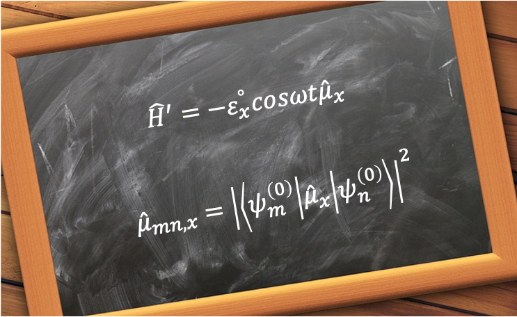Therefore, $q_i\varepsilon_x=-\frac{dV}{dx}$ , whose integrated form is $V=-q_ix\varepsilon_x$ , which is consistent with the classical interaction energy between the electric field and a charged particle. If we consider multiple charges and an oscillating electric field, the perturbation can be expressed approximately as

$\hat{H'} =-\sum_kq_kx_k\varepsilon_x^{\circ}cos\omega t=-\varepsilon_x^{\circ} cos\omega t\hat{\mu}_x\;\;\;\;\;\;\;\;281h$

where $\varepsilon_x^{\circ}$ is the maximum amplitude of the electric field in the $x$ -direction, $\omega=2\pi\nu$ and $\hat{\mu}_x$ is the operator for the $x$ -component of the atom or molecule’s dipole moment, i.e. $\hat{\mu}_x=\sum_kq_kx_k$ .

Question

Why did we not consider the magnetic component of the electromagnetic wave?

Answer

This is because interaction between the magnetic component of the electromagnetic wave and the charges of an atom or molecule is more than a hundred times weaker than interaction between the electric component of the electromagnetic wave and the charges of the atom or molecule.

Substituting eq281h, $\frac{e^{i\omega t}+e^{-i\omega t}}{2}=\frac{cos\omega t+isin\omega t+cos\omega t-isin\omega t}{2}=cos\omega t$ and $\omega_m-\omega_n=\omega_{mn}=\frac{E_m^{(0)}-E_n^{(0)}}{\hbar}$ in eq281g for $m\neq n$ ,

$c_m(t')\approx \frac{i\varepsilon_x^{\circ}}{2\hbar}\int_0^{t'}\langle\psi_m^{(0)}\vert(e^{i\omega t}+e^{-i\omega t})\hat{\mu}_x\vert\psi_n^{(0)}\rangle e^{i\omega_{mn}t}dt$

Since $e^{i\omega t}+e^{-i\omega t}$ is a function of time and not position, it is a constant with regard to the integral with respect to position and we have

$c_m(t')\approx \frac{i\varepsilon_x^{\circ}}{2\hbar}\langle\psi_m^{(0)}\vert\hat{\mu}_x\vert\psi_n^{(0)}\rangle \int_0^{t'}[e^{i(\omega_{mn}+\omega) t}+e^{i(\omega_{mn}-\omega )t}]dt$

$c_m(t')\approx \frac{\varepsilon_x^{\circ}}{2\hbar}\langle\psi_m^{(0)}\vert\hat{\mu}_x\vert\psi_n^{(0)}\rangle \left[\frac{e^{i(\omega_{mn}+\omega)t'}-1}{\omega_{mn}+\omega}+\frac{e^{i(\omega_{mn}-\omega )t'}-1}{\omega_{mn}-\omega}\right]\;\;\;\;\;\;\;\;281i$

When $\omega_{mn}=\omega=2\pi\nu$ , we have $E_m^{(0)}-E_n^{(0)}=h\nu$ , which implies that $\omega_{mn}=\omega$ corresponds to the transition frequency of an atom or molecule from state $n$ to $m$ . Therefore, $\vert c_m(t')\vert^2\propto\vert\langle\psi_m^{(0)}\vert\hat{\mu}_x\vert\psi_n^{(0)}\rangle\vert^2$ is the probability that a measurement of a system will yield an eigenvalue associated with $\psi_m^{(0)}$ after perturbation at $t > t'$ from the state $n$ at $t=0$ ( $\frac{e^{i(\omega_{mn}-\omega )t'}-1}{\omega_{mn}-\omega}$ is not infinite when $\omega_{mn}=\omega$ , see Q&A below). In other words, the transition probability from state $n$ to $m$ of an atom or molecule irradiated by an electromagnetic wave oscillating in the $x$ -direction is proportional to $\vert\langle\psi_m^{(0)}\vert\hat{\mu}_x\vert\psi_n^{(0)}\rangle\vert^2$ , which is denoted by $\mu_{mn,x}$ .

Question

Evaluate $\frac{e^{i(\omega_{mn}-\omega )t'}-1}{\omega_{mn}-\omega}$ when $\omega_{mn}=\omega$ .

Answer

Let $x=\omega_{mn}-\omega$ , with $\frac{e^{i(\omega_{mn}-\omega )t'}-1}{\omega_{mn}-\omega}=\frac{e^{it'x}-1}{x}$ . As $x\rightarrow 0$ , we have $\lim_{x\rightarrow 0}\frac{e^{it'x}-1}{x}$ . Using L’Hopital‘s rule,

$\lim_{x\rightarrow 0}\frac{\frac{d}{dx}(e^{it'x}-1)}{\frac{d}{dx}x}=it'$

For an electromagnetic wave that is not plane-polarised, $\hat{\boldsymbol{\mathit{\mu}}}=\boldsymbol{\mathit{i}}\hat{\mu}_x+\boldsymbol{\mathit{j}}\hat{\mu}_y+\boldsymbol{\mathit{k}}\hat{\mu}_z$ and $\vert c_m(t')\vert^2\propto\vert\langle\psi_m^{(0)}\vert\hat{\boldsymbol{\mathit{\mu}}}\vert\psi_n^{(0)}\rangle\vert^2=\boldsymbol{\mathit{\mu}}_{mn}$ . We called $\boldsymbol{\mathit{\mu}}_{mn}$ the transition dipole moment. In general, transitions are allowed when $\boldsymbol{\mathit{\mu}}_{mn}\neq 0$ , while transitions are forbidden when $\boldsymbol{\mathit{\mu}}_{mn}=0$ .