November 16, 2019 - Mono Mole

November 16, 2019June 16, 2024

Modern atomic structure

The earlier models of the atom were constructed using classical mechanics. When Niels Bohr introduced his model of the atom, he not only utilised Newtonian mechanics in his derivation but also incorporated the Planck relation E = hv, which was conceived a decade earlier by Max Planck, a German physicist.

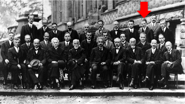
In 1900, Planck was trying to develop a formula to describe the radiation spectrum of a black body when he suggested that electromagnetic radiation is a form of energy that is quantised. The significance of this concept eventually led to development of quantum theory, with Planck being regarded as the father of quantum mechanics.

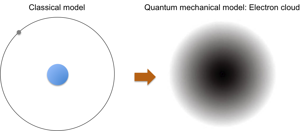
Quantum mechanics is key to the elucidation of the modern structure of an atom, where electrons are no longer perceived as orbiting in defined paths around the nucleus. Instead, an atom is represented by equations that describe the probability distribution of electrons in space, giving rise to a nucleus that is surrounded by an electron cloud (see below diagram).

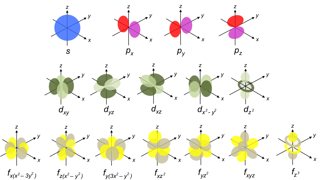
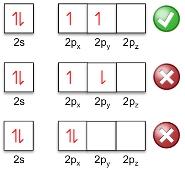
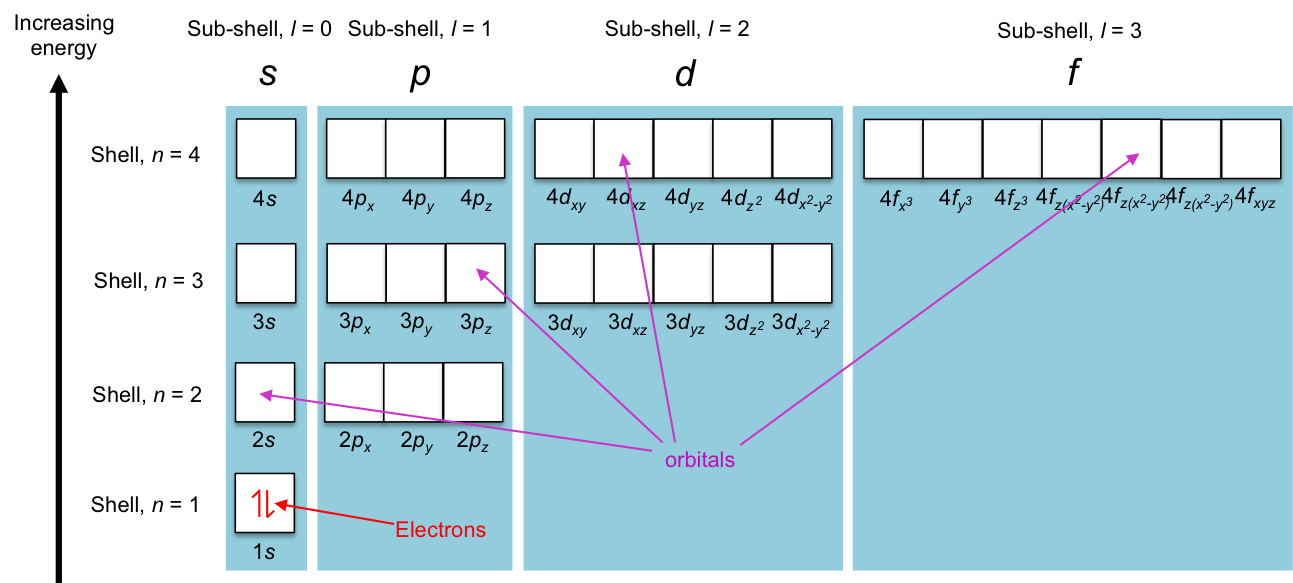
In the modern interpretation of the atomic structure, electrons are distributed in an atom in specific energy states that are characterised by mathematical functions known as orbitals. The maximum number of electrons that an orbital can accommodate is two (see this article for details). Orbitals with similar shapes form a sub-shell (characterised by a unique set of (n, l), e.g. p_x, p_yand p_z forms the sub-shell p), and sub-shells with the same energy in the absence of an external magnetic field, constitute a shell (e.g. 2s and 2p sub-shells constitute the shell n = 2). Diagrammatically, we can describe the energy states as follows:

Mathematically, the energy states are defined by four quantum numbers, n, $l$ , $m_l$ and m_s, as shown in the table below.

Quantum numbers			Details	Example
Symbol	Name	Values	Details	Example
n	Principal	$n\in \mathbb{Z}$ $n\geq 1$	Each value of n refers to a shell	n = 1 and n = 2 are the 1^st shell and 2^nd shell of an atom respectively.
$l$	Angular	$l\in \mathbb{Z}$ $0\leq l\leq n-1$	Each value of $l$ refers to a sub-shell where $\begin{matrix} \; \; \; \; \; \; \; \; \; \; \;\; l: \; \; 0\;\; 1\; \; 2\; \; 3\; ...\\ Subshell:\; s\; \; p\;\; d\; \; f\; ... \end{matrix}$	For the 1^st shell (n = 1), $l=0$ , i.e. the 1^st shell consists only of the sub-shell s. For the 2^nd shell (n = 2), $0\leq l\leq 1$ , i.e. the 2^nd shell consists of two sub-shells, s and p.
$m_l$	Magnetic	$m_l\in \mathbb{Z}$ $-l\leq m_l\leq l$ with a total of $2l+1$ values	Each value of $m_l$ refers to the orientation of an orbital in a sub-shell. The total number of $m_l$ values in a sub-shell also refers to the total number of orbitals in that sub-shell.	For the 1^st shell (n = 1), $l=0$ , and $m_l=0$ , with a total of one $m_l$ value, i.e. there is only one orbital in the 1^st shell. For the s sub-shell in the 2^nd shell, $m_l=0$ with a total of one $m_l$ value, i.e. there’s only 1 orbital in the s sub-shell with a single orientation. For the p sub-shell in the 2^nd shell, $-1\leq m_l\leq 1$ with a total of three $m_l$ values, i.e. 3 orbitals in the p sub-shell, with each orbital having a distinct orientation.
$m_s$	Spin magnetic	$+\frac{1}{2}$ or $-\frac{1}{2}$	Each value of $m_s$ refers to the spin orientation of an electron.	$+\frac{1}{2}$ refers to a spin-up electron, while $-\frac{1}{2}$ refers to a spin-down electron

In other words, the four quantum numbers describe the energy state of an electron in an atom. The numbers are a result of many scientists’ work that were done during the early 1900s. Some of these experiments and theories that contributed to the development of quantum mechanics are listed in the table below.

Year	Work	Scientist
1900	Planck’s law	Max Planck
1905	Photoelectric effect	Albert Einstein
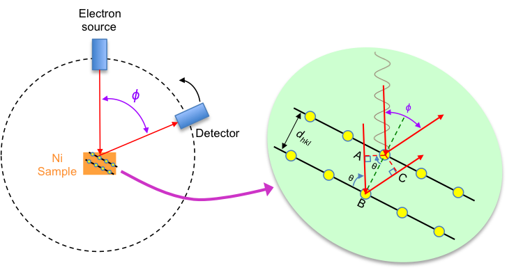
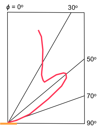
1924	de Broglie’s hypothesis	Louis de Broglie
1925	Schrodinger equation	Erwin Schrodinger
1925	Pauli exclusion principle	Wolfgang Pauli
1926	Born interpretation	Max Born
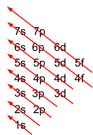
1920-1930	Aufbau principle, Madelung’s rule and Hund’s rule	Niels Bohr, Wolfgang Pauli, Erwin Madelung, Friedrich Hund
1927	Heisenberg’s uncertainty principle	Werner Heisenberg

We shall elaborate on the above in the following articles.

Question

Does the energy level diagram for shells and sub-shells apply to all atoms?

Answer

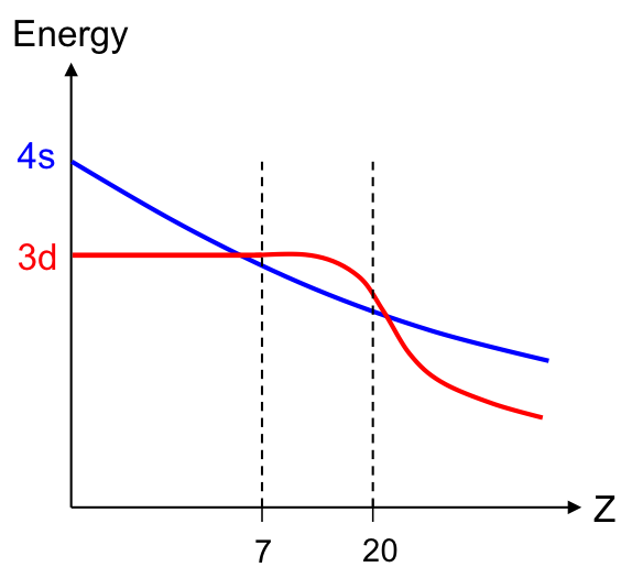
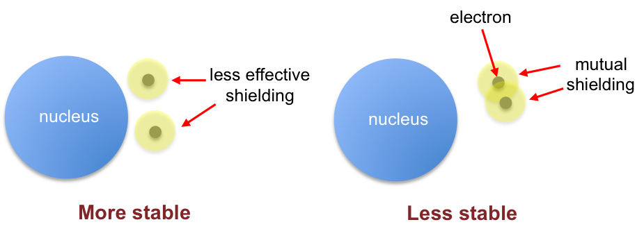
The above energy level diagram is a result of the solution of the Schrodinger equation for the hydrogen atom, which has degenerate sub-shells, i.e. sub-shells belonging to a particular shell (e.g. 2s and 2p for n = 2) have the same level of energy. The degeneracy of sub-shells disappears for multi-electron atoms due to electron-electron repulsion and the shielding effect of orbitals. For a particular shell in a multi-electron atom, the smaller the angular quantum number, the lower the energy level of the sub-shell within that shell.

Next article: Black body radiation

Previous article: Classical atomic theory

Content page of intermediate quantum chemistry

Content page of intermediate chemistry

Main content page

November 16, 2019May 4, 2024

de Broglie’s hypothesis

The de Broglie’s hypothesis states that all matter exhibits characteristics of both wave and particle. It was developed by Louis de Broglie, a French physicist, in 1924 without any experimental evidence.

What inspired him was Planck’s and Einstein’s work, which collectively proposed that light has the properties of a particle with a quantised energy of hv, in addition to the properties of a wave as previously proven by Thomas Young in his famous double-slit experiment.

de Broglie used Planck’s relation E = hv and Einstein’s mass-energy equivalence formula E = mc² to establish the de Broglie relation:

$hv=mc^2$

$hv=pc\; \; \; \; \; \; \; \; 3$

where p = mc is the relativistic momentum of a photon.

Substituting the relation c = vλ in eq3:

$p=\frac{h}{\lambda}\; \; \; \; \; \; \; \; 4$

which is de Broglie’s relation.

de Broglie suggested that if light exhibited both wave (wavelength) and particle (momentum) characteristics, then all particles would have both properties as well. The soundness of de Broglie’s hypothesis was subsequently verified by experiments, most notably the Davisson-Germer experiment.

Question

Why is c = vλ?

Answer

Frequency v is the number of complete waves that passes a point per second and so, the inverse of frequency is the time for a single complete wave to pass through a point. Wavelength λ is the distance over which a complete wave repeats. Therefore, the speed of a wave is λ/(1/v) = vλ.

The implication of the de Broglie relation is that all matter has wave-like properties. For example, a 70kg person running with a speed of 4 m/s has a wavelength of 2.4 x 10^-36 m. However, the wavelength is too small for any wave phenomenon to be observed, e.g. the person doesn’t undergo diffraction as he runs through an open door.

The de Broglie relation is a significant development in the field of quantum mechanics and is consistent with the Schrodinger equation, which quantum mechanically describes the motion of an electron in a way analogous to Newton’s laws of motion that classically describes the motion of objects.

Next article: davisson-Germer experiment

Previous article: Photoelectric effect

Content page of intermediate quantum chemistry

Content page of intermediate chemistry

Main content page

November 16, 2019April 3, 2023

Davisson-Germer experiment

The Davisson-Germer experiment studies the scattering of electrons by a nickel single crystal. In 1927, Clinton Davisson and Lester Germer, both American physicists, irradiated a nickel single crystal with a 54 eV electron beam* and rotated the detector at various angles to capture the scattered electrons (see below diagram).

* The electron beam energy of 54 eV or 8.65 x 10^-18 J is attributed to the kinetic energy of an electron (see this article for details).

Prior to the experiment, an electron is known to be a particle with a mass of 9.1 x 10^-31 kg. In 1924, de Broglie hypothesised that electrons also possess wave characteristics. If so, and if electrons have wavelengths similar to the interatomic distance (or interplannar distance) of nickel in the experiment, they would be diffracted by the nickel crystal, resulting in interference patterns typically seen in Thomas Young’s diffraction experiments.

The results indeed produced such a diffraction pattern, with a first-order constructive interference peak at φ = 50° (see diagram above). According to Bragg’s law,

$2dsin\theta=n\lambda\; \; \; \; \; \; \; \; 5$

where d is the interplannar distance and n is the order of diffraction.

With reference to the top diagram, $\theta=90^o-\frac{\phi}{2}$ . Substituting $\theta=90^o-\frac{50^o}{2}=65^o$ , the interplannar distance of Ni of 91 pm and n = 1 in eq5, the wavelength of the electron is λ = 165 pm.

To test de Broglie’s hypothesis, we rearrange de Broglie’s relation as follows:

$\lambda=\frac{h}{p}=\frac{h}{mv}=\frac{h}{\sqrt{2m\left ( \frac{1}{2}mv^2 \right )}}=\frac{h}{\sqrt{2m(KE)}}\; \; \; \; \; \; \; \; 6$

Substituting the value of the Planck constant (6.62 x 10^-34 m²kg s^-1), the mass of an electron (9.1 x 10^-31 kg) and kinetic energy of an electron (54 eV = 8.65 x 10^-18 J ) in eq6, we get λ = 167 pm, which is in very close agreement with the experimental value of 165 pm.

The Davisson-Germer experiment therefore verifies the wave characteristic of electrons and de Broglie’s hypothesis.

Subsequently, other experiments involving other elementary particles, atoms and even macromolecules like C₆₀ were conducted, all of which, validated de Broglie’s hypothesis. The technique employed by Davisson and Germer is now known as low energy electron diffraction (LEED), which is utilised to study surface properties of material.

Next article: Schrodinger equation

Previous article: de Broglie’s hypothesis

Content page of intermediate quantum chemistry

Content page of intermediate chemistry

Main content page

November 16, 2019October 12, 2023

The Born interpretation

The Born interpretation states that the probability of finding an electron of a certain quantum state around a point is proportional to the square of the modulus of the electron’s wave function $\left | \psi \right |^2$ , which is called the probability density. It was proposed by Max Born, a german Physicist, in 1926.

In developing the concept, Born drew a parallel between the probability of finding a particle in a region of space and the intensity of a classical wave, which is proportional to the square of the wave’s amplitude.

Question

Using Hooke’s law, F = –kx, show that the intensity of a wave is proportional to the square of its amplitude.

Answer

Substituting Hooke’s law in dE = –Fdx, we have dE = kxdx (where E is energy). Integrating the simple harmonic motion over a maximum amplitude A,

$E=\int_{0}^{A}kxdx=\frac{1}{2}kA^2$

Since intensity I is defined as $\frac{energy}{time\times area}$ , we have $I\propto E\propto A^2$ for an electromagnetic radiation falling on a particular area of a material over a certain duration.

Mathematically, the Born interpretation is:

$\int \left | \psi \right |^2d\tau$

or $\int \left | \psi \right |^2d\tau=1$ to ensure that the sum of individual probabilities of locating an electron over all space is normalised to one. The wave function of an electron is a complex quantity and therefore the above equation can be written as:

$\int \psi^*\psi d\tau$

where $\psi^*$ is the complex conjugate of $\psi$ .

Question

Why is the wave function a complex quantity? Show that $\psi^*\psi=\left | \psi \right |^2$ .

Answer

Some differential equations are easier to solve when the function is in the complex form. This happens to be the case for the Schrodinger equation. However, only the real component is used when values of the function are compared with experimental data.

Let $\psi=a+ib$ . So $\left | \psi \right |=\sqrt{a^2+b^2}\; \; \Rightarrow \; \; \left | \psi \right |^2=a^2+b^2$ .

$\psi^*\psi=(a-ib)(a+ib)=a^2+b^2$

Therefore, $\psi^*\psi=\left | \psi \right |^2$ .

In the previous article, we mentioned that Schrodinger did not have a convincing physical interpretation of the wave function ψ, other than it being a wave equation of an electron in the atom. With the Born interpretation, the electron probability density function $\left | \psi \right |^2$ for a unique combination of the three quantum numbers $n$ , $l$ and $m_l$ , mathematically describes an atomic orbital. When we plot the probability functions using a mathematical software, we obtain the following shapes:

These are the orbitals of a hydrogen atom.

Next article: Electron spin

Previous article: Schrodinger equation

Content page of intermediate quantum chemistry

Content page of intermediate chemistry

Main content page

November 16, 2019April 16, 2023

Electron spin

Ever since scientists recorded the first hydrogen emission spectrum, they produced many significant findings, including the Balmer and Lyman series, the Rydberg formula and the Bohr model. However, when researchers scrutinised the spectrum under magnification, they discovered that the emission line from n = 2 to n = 1 consisted of two lines (see diagram below).

This splitting of emission lines is called the hydrogen fine structure. Many attempts were made to explain this phenomenon without success. At around 1924, Wolfgang Pauli, an Austrian physicist, and two other scientists (George Uhlenbeck and Samuel Goudsmit, both Dutch scientists), separately proposed that an electron possesses an intrinsic property called spin. Even though the spin of an electron is strictly a quantum mechanical property, it is possible to shed light on the concept using classical electromagnetism, where the electron is spinning on its own axis, while orbiting around the nucleus.

According to the classical model, a flow of charges generates a magnetic field, whose direction is given by the right-hand rule. An electron orbiting in a clockwise direction (when viewed from the top) around the nucleus of an atom therefore possesses a magnetic (orbital) dipole moment $\mu_l$ (see diagram below).

The electron spinning on its own axis in a clockwise direction has another magnetic (spin) dipole moment $\mu_s$ , because a spinning charge produces an effective current loop. Since the two dipole moments are vectors, they interact with each other to give an effective dipole moment. This ‘spin moment’-‘orbital field’ interaction is called spin-orbit coupling. If the allowed spin orientations are such that the magnetic spin dipole moments are either parallel or anti-parallel to the magnetic orbital dipole moment, the spin-orbit couplings will result in two quantum states of different energies.

Question

What is a magnetic dipole moment?

Answer

According to classical electromagnetic theory, a moving charge generates a magnetic field, which implies the presence of north and south magnetic poles called a magnetic dipole. The magnetic dipole moment is a measure of the strength and orientation of a magnetic dipole, i.e. a vector.

This is the reason why an electron, when excited to the n = 2 shell of the hydrogen atom, has one of two possible states (energy levels), namely ²P_3/2 and ²P_1/2. When the electron relaxes back to the n = 1 shell, one of two emission lines is observed, depending on whether the electron was initially promoted to the upper or lower state. The concept of electron spin and quantised spin orientations are validated by the Stern-Gerlach experiment, where a beam of silver atoms is directed through a magnetic field gradient.

In solving the Schrodinger equation for the hydrogen atom, the quantum number $l$ is attributed to the angular momentum of the electron as it orbits the nucleus. Since a particle possesses angular momentum, whether orbiting or spinning, a spinning electron has spin angular momentum. Furthermore, we know from the solution of Schrodinger’s equation that each value of $l$ (a vector) is associated with orientations of the magnetic number $m_l$ , where $m_l=-l,-l+1...0...l-1,l$ . With that, Pauli proposed a fourth quantum number $m_s$ , the spin magnetic number, to fully describe the quantum state of a system. Like $m_l$ , $m_s=-s,-s+1...0...s-1,s$ . The value of $s$ (another vector) was later experimentally determined to be $\frac{1}{2}$ . Therefore, $s$ has two possible orientations of $m_s=-\frac{1}{2}\; or\; +\frac{1}{2}$ .

Question

Shouldn’t the n = 1 shell split into two energy levels too?

Answer

The explanation above provides a qualitative picture of spin-orbit coupling. Mathematically, the spin-orbit interaction energy is computed using the formula:

$E=\frac{1}{2}hcA[j(j+1)-l(l+1)-s(s+1)]$

where h, c and A are constants, and j is the total angular momentum quantum number (i.e. the vector sum of $l$ and $s$ ). For the hydrogen atom, $j=l+s$ and $j=\left | l-s \right |$ .

According to the solution of the Schrodinger equation, when $n=1$ , we have $l=0$ , which makes j = s. Substituting these values in the above equation, we have a single value of E = 0. This means that there is no effect of spin-orbit coupling on the quantum state of n = 1. Using the same logic, we find that the quantum state for $n=2,l=1$ gives two values of E of $\frac{1}{2}hcA$ and $-\frac{1}{2}hcA$ , which when added to the energy of the quantum state of “ $n=2,l=1$ “, results in the states ²P_3/2 and ²P_1/2.

Next article: Pauli exclusion principle

Previous article: The Born interpretation

Content page of intermediate quantum chemistry

Content page of intermediate chemistry

Main content page

November 16, 2019August 25, 2023

Pauli exclusion principle

The Pauli exclusion principle states that it is not possible for two electrons in an atom to have the same set of quantum numbers.

Wolfgang Pauli, an Austrian physicist, developed this principle in 1925, after considering evidences and proposals put forward by scientists in the early 1900s. These evidences and proposals include:

- Atoms with even numbers of electrons are relatively stable as compared to those with odd numbers of electrons.
- The maximum number of electrons a shell holds is an even one. Such a shell is called a closed shell.
- The number of electrons in closed shells is 2, 8 and 18 for n = 1, n = 2 and n = 3 respectively.

From the solutions of the Schrodinger equation for the hydrogen atom, the three quantum numbers $n$ , $l$ and $m_l$ are integers, with $n\geq 1$ , $0\leq l\leq n-1$ and $-l\leq m_l\leq l$ . Therefore, we have

${\color{Red} n}$	${\color{Red} l}$	${\color{Red} m_l}$	${\color{Red} Total\, m_l\, count}$
1	0	0	1
2	0, 1	0 and -1, 0, +1	4
3	0, 1, 2	0 and -1, 0, +1 and -2, -1, 0, +1, +2	9

Comparing the total $m_l$ count and the total number of electrons in the first three closed shells, every $m_l$ corresponds to an average of two electrons. If we associate each value of $m_l$ with an orbital and assume an equal distribution of electrons among orbitals to achieve a stable state of minimum energy, each orbital can accommodate a maximum of two electrons. As mentioned in the previous article, Pauli introduced a fourth quantum number called the spin magnetic number $m_s$ , which is related to the orientation of electrons in an atom, to fully describe the quantum state of the atom. Furthermore, the solution of the Schrodinger equation results in a zero probability of two electrons with parallel spins residing in the same orbital. It is therefore logical to assume that the relative stability exhibited by atoms with even number of closed-shell electrons is due to an anti-parallel orientation of an electron pair in each orbital. This implies that no two electrons in an atom can be described by the same set of quantum numbers. For example, the electron configuration of helium in the ground state is:

where the quantum state of one electron is $n=1,l=0,m_l=0,m_s=+\frac{1}{2}$ or $\left ( 1,0,0,+\frac{1}{2} \right )$ , while the quantum state of the other electron is $n=1,l=0,m_l=0,m_s=-\frac{1}{2}$ or $\left ( 1,0,0,-\frac{1}{2} \right )$ . In other words, the Pauli exclusion principle states that

Each atomic orbital can hold a maximum of two electrons and that two electrons in the same orbital must have anti-parallel spins.

Next article: Aufbau principle

Previous article: Electron spin

Content page of intermediate quantum chemistry

Content page of intermediate chemistry

Main content page

November 16, 2019April 21, 2023

Schrodinger equation

The Schrodinger equation is a partial differential equation, whose solutions are wave functions that describe the quantum states of a system. It was formulated by Erwin Schrodinger in 1925, after de Broglie published his hypothesis, which proposed that all matter have wave-like properties.

Schrodinger reckoned that if electrons behave like waves, they could be described by a wave equation. This eventually led to the time-independent Schrodinger equation in one-dimension:

$\hat{H}\psi=E\psi$

where $\hat{H}=-\frac{\hbar^2}{2m}\frac{\partial^2}{\partial x^2}+V(x)$ and $\hbar=\frac{h}{2\pi}$ .

$\hat{H}$ is called the Hamiltonian operator, E is the total energy of the system and V is the potential energy of the system. Solutions to the equation are different expressions of ψ, the wave function. In terms of linear algebra, the Schrodinger equation is an eigenvalue equation; ψ is an eigenfunction and E is the corresponding eigenvalue. It is regarded as a postulate, meaning it is so fundamental that it cannot be derived.

Question

What is a postulate and how did Schrodinger arrive at the equation if it cannot be derived?

Answer

A postulate is a statement that everyone agrees is true. It is so fundamental that it cannot be proven. Examples of postulates include Newton’s 2^nd law, F = ma, and the Euclidean statement that a line is defined by two points. Although we cannot derive the Schrodinger equation, we can show that it is consistent with the concept of energy conservation and de Broglie’s relation by substituting a simple wave function $\psi=cos\frac{2\pi}{\lambda}x$ into the equation:

$-\frac{\hbar^2}{2m}\frac{\partial^2}{\partial x^2}\left ( cos\frac{2\pi}{\lambda}x \right )+V(x)\left ( cos\frac{2\pi}{\lambda}x \right )=E\left ( cos\frac{2\pi}{\lambda}x \right )$

which computes to

$\frac{h^2}{2m\lambda^2}=E-V(x)$

Since is E – V(x) the kinetic energy of the system,

$\frac{h^2}{2m\lambda^2}=\frac{p^2}{2m}\; \; \Rightarrow \; \; p=\frac{h}{\lambda}$

which is the de Broglie relation.

For a three-dimensional system, the Hamiltonian is:

$\hat{H}=-\frac{\hbar^2}{2m}\left ( \frac{\partial^2}{\partial x^2}+\frac{\partial^2}{\partial y^2}+\frac{\partial^2}{\partial z^2}\right )+V(x,y,z)$

The process of solving the equation for an atom is a tedious one. However, a complete set of solutions can be derived algebraically for the hydrogen atom, with each solution given by the general wave function:

$\psi(r,\theta,\phi)=R(r)Y(\theta,\phi)$

where

$R(r)=\sqrt{\left ( \frac{2}{a_0n} \right )^3\frac{(n-l-1)!}{2n(n+l)!}}\: e^{-\frac{r}{a_0n}}\left ( \frac{2r}{a_0n} \right )^lL_{n-l-1}^{2l+1}\left ( \frac{2r}{a_0n} \right )$

$Y(\theta,\phi)=\frac{1}{\sqrt{2\pi}}\left [ \left ( \frac{2l+1}{2} \right )\frac{\left ( l-\left | m_l \right | \right )!}{\left ( l+\left | m_l \right | \right )!} \right ]^{\frac{1}{2}}P_l^{\left | m_l \right |}(cos\theta) e^{im_l\phi}$

$L_{n-l-1}^{2l+1}=\sum_{k=0}^{n-l-1}(-1)^k\frac{(n+l)!}{k!(n-l-1-k)!(k+2l+1)!}\left ( \frac{2r}{a_0n} \right )^k$

$P_l^{\left | m_l \right |}(cos\theta)=\left ( 1-cos^2\theta \right )^{\frac{\left | m_l \right |}{2}}\left [ \frac{d^{\, l+\left | m_l \right |}}{dcos\theta^{\, l+\left | m_l \right |}}\left ( cos^2\theta-1 \right )^l \right ]$

R(r) and Y(θ, φ) are the radial component and angular component of the wave function respectively. $L_{n-l-1}^{2l+1}$ is the associated Laguerre polynomial and $P_l^{\left | m_l \right |}(cos\theta)$ is the associated Legendre function.

While solving the Schrodinger equation, three quantum numbers, n, l and m, which can be seen in the radial component and angular components of the wave function, are defined. The solutions require the quantum numbers to have values stated in the following table:

Quantum numbers
Symbol	Name	Values
n	Principal	$n\in \mathbb{Z}$ , $n\geq 1$
$l$	Angular	$l\in \mathbb{Z}$ , $0\leq l\leq n-1$
$m_l$	Magnetic	$m_l\in \mathbb{Z}$ , $-l\leq m_l\leq n-1$ with a total of $2l+1$ values

We have seen the principal quantum number n before, in the Bohr model. Each value of n refers to a shell. The angular quantum number $l$ is associated with the angular momentum of an electron and designates a subshell. The magnetic quantum number $m_l$ is the projection of the angular momentum vector of the electron on the z-axis. The possible combinations of these three numbers specify the quantum states (energy states) of the atom. Despite the solutions for the hydrogen atom, Schrodinger did not have a convincing physical interpretation of the wave function ψ, other than it being a wave equation of an electron in the atom. Then came Max Born.

Next article: The Born interpretation

Previous article: davisson-Germer experiment

Content page of intermediate quantum chemistry

Content page of intermediate chemistry

Main content page

November 16, 2019April 16, 2023

Aufbau principle

The Aufbau principle (building up principle) states that an atom in the ground state has electrons filling its orbitals in the order of increasing energy. It was proposed by Niels Bohr and Wolfgang Pauli in the 1920s and is based on the observation that the lower the energy of a system is, the more stable it is.

Specifically, the principle adopts the $n+l$ rule, which was first suggested by Charles Janet in 1928, in his attempt to construct a version of the periodic table. It was later adopted by Erwin Madelung in 1936, as a rule on how atomic sub-shells are filled.

The empirical rule states that electrons fill sub-shells in the order of increasing value of $n+l$ where $n$ is the principal quantum number and $l$ is the angular quantum number. It further mentions that electrons fill sub-shells in the order of increasing value of $n$ for sub-shells with identical values of $n+l$ . For example,

Subshell	${\color{Red} n}$	${\color{Red} l}$	${\color{Red} n+l}$	Order
1s	1	0	1	1
2s	2	0	2	2
2p	2	1	3	3
3s	3	0	3	4
3p	3	1	4	5
3d	3	2	5	7
4s	4	0	4	6

The order of fill is represented by the diagram above. So, the ground state electron configuration (distribution of electrons) for calcium is 1s² 2s² 2p⁶ 3s² 3p⁶ 4s² or [Ar]4s², where [Ar] is the electron configuration of argon. The Aufbau principle works well for elements with atomic number $Z\leq 20$ but must be applied with a better understanding of orbital energy and electron repulsion for $Z>20$ .

For elements with Z between 1 and 6, calculations show that the energy of the 4s sub-shell is higher than the 3d sub-shell (see diagram above). For Z between 7 and 20, the reverse is true, as a result of the interplay between increasing nuclear charge and increasing electron repulsion. The relative energy of the s and d sub-shells again changes for $Z>20$ , where the 3d sub-shell has a lower energy than the 4s sub-shell. This is because electrons in 3d orbitals do not shield each other well from nuclear forces, leading to the lowering of their energies.

With that in mind, one may conclude that the electron configurations of scandium and titanium are [Ar]3d³and [Ar]3d⁴ respectively. However, they are [Ar]3d¹4s²and [Ar]3d²4s². Numerical solutions of the Schrodinger equation for scandium and titanium not only show that the 3d orbitals have lower energies than the 4s orbitals, but also reveal that the 3d orbitals are smaller in size compared to the 4s orbitals. Electrons occupying 3d orbitals therefore experience greater repulsions than electrons residing in 4s orbitals, with the order of increasing repulsion being:

$V\left ( e_{4s},e_{4s} \right )<V\left ( e_{4s},e_{3d} \right )<V\left ( e_{3d},e_{3d} \right )$

where V is the potential energy due to repulsion.

To determine the stability of an atom in the ground state, we need to consider the net effect of the relative energies of 4s/3d orbitals and the repulsion of electrons. In fact, calculations for the overall energies of scandium are as follows:

$E[Ar]3d^14s^2<E[Ar]3d^24s^1<E[Ar]3d^3$

Consequently, when a transition metal undergoes ionisation, the electron is removed from the 4s orbital rather than the 3d sub-shell. Despite 3d being lower in energy than 4s for the first row of transition metals, the $n+l$ rule applies. However, the rule breaks down for chromium and copper, where the ground state electronic configuration of chromium is [Ar]3d⁵4s¹instead of [Ar]3d⁴4s² and that of copper is [Ar]3d¹⁰4s¹ instead of [Ar]3d⁹4s². This is attributed to Hund’s rule.

Next article: Hund’s rule

Previous article: Pauli exclusion principle

Content page of intermediate quantum chemistry

Content page of intermediate chemistry

Main content page

November 16, 2019April 16, 2023

Hund’s rule

Hund’s rule states that electrons occupy orbitals of a sub-shell singly and in parallel before pairing up (see diagram below for the n = 2 shell of carbon). This is sometimes called the ‘bus seat’ rule, where bus passengers who travel alone tend to occupy empty double-seats before partly occupied seats.

By spacing themselves apart in different orbitals, electrons attain a relatively stable configuration. This is because electrons offer one another less shielding from the nuclear charge if they are further apart. The decreased shielding leads to the electrons being stabilised closer to the nucleus, resulting in a lower energy system (see digram below).

But why do the electrons that occupy the p-orbitals singly in the above example have parallel spins? A crude explanation is to visualise an electron with a north pole and a south pole (a dipole) due to the magnetic field that it generates with its spin. To stay far apart from each other to reduce repulsion, the dipoles of the two electrons in the p sub-shell must be aligned in a parallel fashion. If the dipoles are anti-parallel, the electrons will be closer to each other, resulting in a higher and less stable energy state. The proper explanation for Hund’s rule, however, lies in the symmetry of the wave function of the system.

Question

Why can’t the n = 2 electron configuration of carbon be 2s¹2p_x¹2p_y¹2p_z¹?

Answer

The stability of the ground state of carbon is a result of the interplay between Hund’s rule and the Aufbau principle. Since the 2s orbital is of a lower energy than each of the 2p orbitals, the electron configuration of the n = 2 shell of 2s²2p_x¹2p_y¹2p_z⁰ offers greater stability to the system than the configuration of 2s¹2p_x¹2p_y¹2p_z¹.

To understand why the ground state electron configuration of chromium is [Ar]3d⁵4s¹instead of [Ar]3d⁴4s²and that of copper is [Ar]3d¹⁰4s¹instead of [Ar]3d⁹4s², we need to consider the following:-

1. The 3d sub-shell has a lower energy than the 4s sub-shell for Z > 20 (see previous article).
2. Electrons occupying 3d orbitals experience greater repulsions than electrons residing in 4s orbitals (see previous article).
3. Hund’s rule states that electrons prefer to stay apart from one another by occupying orbitals singly before pairing up.

The electronic configuration of a 1^st row transition metal is dependent on the interplay of the above three factors. For chromium, the energy level of the 3d sub-shell is very close to that of the 4s sub-shell and hence the 3^rd factor outweighs the 2^nd one. For copper, the energy level of the 3d sub-shell is much lower than that of the 4s sub-shell such that the 1^st factor outweighs the other two factors.

Next article: Heisenberg’s uncertainty principle

Previous article: Aufbau principle

Content page of intermediate quantum chemistry

Content page of intermediate chemistry

Main content page

November 16, 2019April 16, 2023

Heisenberg’s uncertainty principle

Heisenberg’s uncertainty principle states that the position and momentum of a particle cannot be determined simultaneously with unlimited precision. It was developed by Werner Heisenberg, a German physicist, in 1927 and is expressed mathematically as:

$\Delta p_x\Delta x\geq \frac{\hbar}{2}$

where $\Delta p_x$ is the uncertainty in the x-component of a particle’s momentum, $\Delta x$ is the uncertainty in the particle’s position along the x-axis, and $\hbar=\frac{h}{2\pi}$ .

In other words, the product of the uncertainty in measuring a particle’s momentum and the uncertainty in the simultaneous measuring of the particle’s position is never less than $\hbar/2$ (see here for proof). It is important to note that the uncertainties in the measurements are not due to the limitation of measuring devices but an inherent property of nature.

To explain the uncertainty principle, we turn to de Broglie’s hypothesis, which states that all matter behaves like waves. For an electron, its wave property is described by a wave function, e.g. $\psi=Ae^{ikx}$ , which has a well-defined wavelength $\lambda=\frac{2\pi}{k}$ (since $Ae^{ik\left ( x+\frac{2\pi}{k} \right )}=Ae^{ikx}$ ) and hence a precisely determined momentum $p=\frac{h}{\lambda}=k\hbar$ . Furthermore, the position of the electron, according to the Born interpretation, is given by the probability density $\left | \psi \right |^2$ where

$\left | \psi \right |^2=\psi^*\psi=Ae^{-ikx}Ae^{ikx}=A^2$

The equation above shows that the probability density of the electron is uniform, i.e. the electron has equal probability to be found anywhere along the x-axis. If an electron’s momentum is precisely specified, its location cannot simultaneously be determined.

For the reverse argument, where the position is precisely defined, let’s start with an electron with a wave function, where the wavelength is precisely defined, e.g. $cos\pi x$ (represented by the red curve in diagram I below).

If we linearly add another wave function with a different wavelength $cos2\pi x$ to $cos\pi x$ and divide the sum by two* to maintain the same amplitude as $cos\pi x$ , we have a new wave function $y=\frac{1}{2}cos\pi x+\frac{1}{2}cos2\pi x$ or $\sum_{n=1}^{N}\frac{cosn\pi x}{N}$ where N = 2. This is equivalent to the interference pattern of two superimposed wave functions. If we continue to superimpose the first wave function with more wave functions, each of different wavelength, we end up with the blue curve, the green curve and the black curve, for N =5, N = 20 and N = 100 respectively. It is evident from diagram I that as more wave functions of different wavelengths are linearly added to the first wave function, the spread of the resultant wave function becomes narrower.

* this is done for convenience, so that the resultant curve can fit within our view.

For the N = 5 wave function, the probability of locating the electron within a certain percentage P is $\int \left | \psi \right |^2dx$ , which is the area under the blue curve from x₅ to x+Δx₅ (diagram II). Notice that all curves in diagram II are above the x-axis since they represent the square of the respective wave functions. For the N = 20 wave function, let’s assume that the probability of locating the electron within the same percentage is approximately the area under the green curve from x₂₀ to Δx₂₀ in diagram III (note that the amplitude of the N = 20 function in the diagram is normalised for convenience; rightfully, it is very much higher than the amplitude of the N =5 function, and hence the areas under both peaks are comparable). Clearly, the interval x₂₀ to x+Δx₂₀ is shorter than the interval x₅ to x+Δx₅. Hence, we can locate the electron, with a certain probability P, within a smaller interval as N increases, i.e. the uncertainty in locating the electron becomes smaller as N increases. However, the resultant wave functions of N =5 and N = 20 now consist of 5 and 20 distinct wavelengths respectively. Since each wavelength represent a specific value of momentum, a wave function with a wider spread of wavelengths leads to a greater uncertainty of momentum. In the limit of N → ∞ , we have a precisely localised electron but a completely unpredictable momentum.

Question

The speed of an electron in a one-dimensional space is measured, within 3% accuracy, as 2.20 x 10⁶ m/s. What is the length of the space?

Answer

The minimum uncertainty in the position of the electron is:

$\Delta x\geq \frac{\hbar}{2m\Delta v_x}=\frac{1.055\times10^{-34}}{2\times9.11\times10^{-31}\times0.03\times2.20\times10^6}=8.8\times10^{-10}\, m$

If we assume that there is absolute certainty that the electron is not outside the region of space, the uncertainty in position of the electron must be attributed to the length of space.

Question

Answer

Next article: Black body radiation

Previous article: Classical atomic theory

Question

Answer

Next article: davisson-Germer experiment

Previous article: Photoelectric effect

Next article: Schrodinger equation

Previous article: de Broglie’s hypothesis

Question

Answer

Question

Answer

Next article: Electron spin

Previous article: Schrodinger equation

Question

Answer

Question

Answer

Next article: Pauli exclusion principle

Previous article: The Born interpretation

Next article: Aufbau principle

Previous article: Electron spin

Question

Answer

Next article: The Born interpretation

Previous article: davisson-Germer experiment

Next article: Hund’s rule

Previous article: Pauli exclusion principle

Question

Answer

Next article: Heisenberg’s uncertainty principle

Previous article: Aufbau principle

Question

Answer

Next article: Nuclear spin

Previous article: Hund’s rule