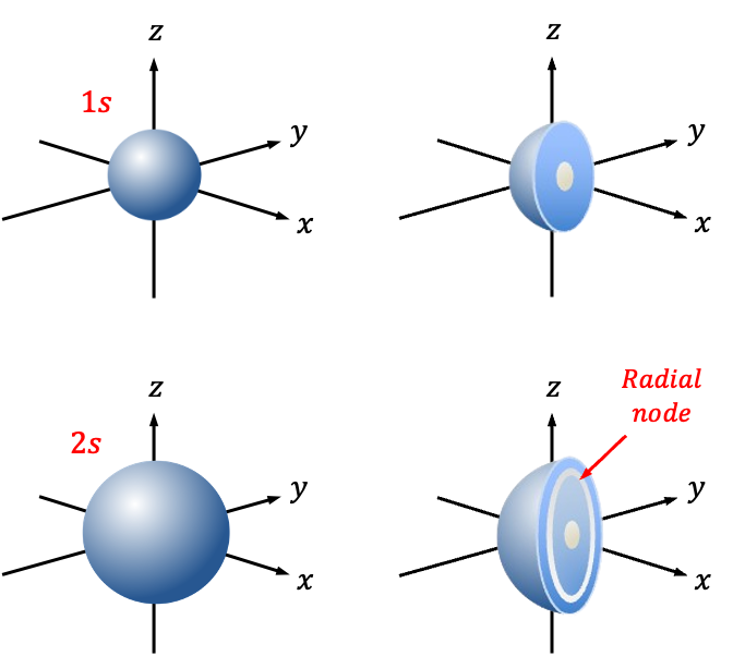
The radial wavefunction ) describes the probability distribution of the distance between an electron and the nucleus of a hydrogenic atom.
describes the probability distribution of the distance between an electron and the nucleus of a hydrogenic atom.
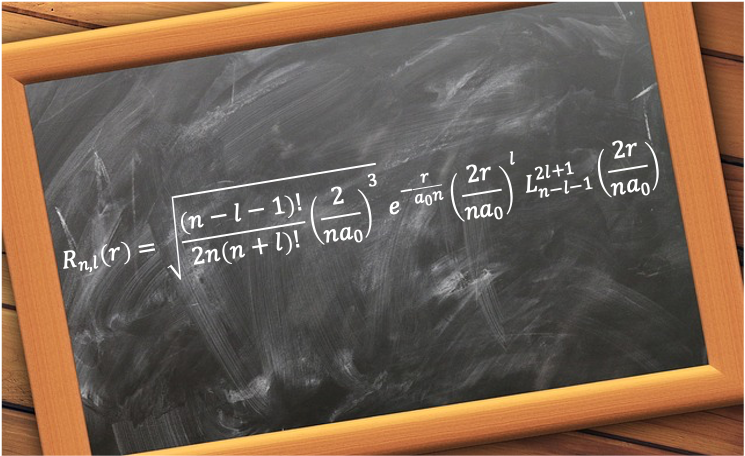
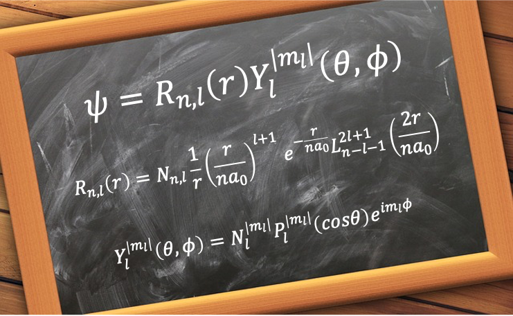
It is given by
=\sqrt{\frac{(n-l-1)!}{2n(n+l)!}\biggr\(\frac{2}{na_0}\biggr\)^3}e^{-\frac{r}{a_0n}}\biggr\(\frac{2r}{na_0}\biggr\)^lL_{n-l-1}^{2l+1}\biggr\(\frac{2r}{na_0}\biggr\)\;\;\;\;\;\;\;\;458)
where
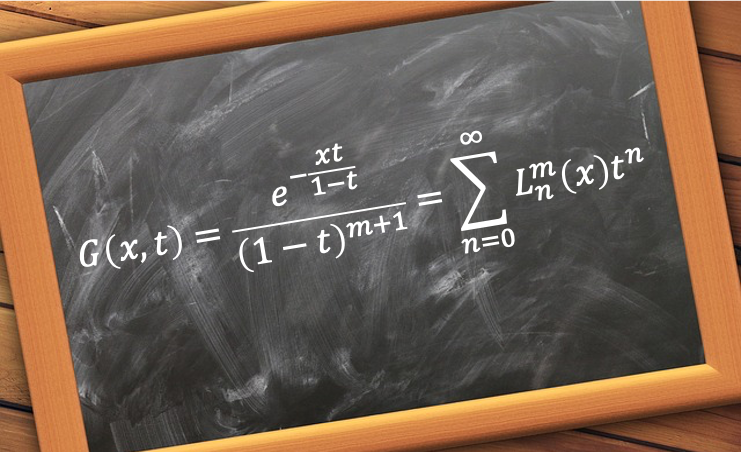
 are the associated Laguerre polynomials.
 is the principal quantum number.
 is the orbital angular momentum quantum number
 is the Bohr radius.
 is the distance between an electron and the nucleus of a hydrogenic atom.

Question
What is a hydrogenic atom?
Answer
It is an atom with only one electron, regardless of the number of protons in its nucleus, making it similar to a hydrogen atom in terms of its electronic structure. Examples of hydrogenic atoms include the hydrogen atom, He+, Li2+ and others.
To derive the un-normalised form of eq458, consider the Schrodinger equation of a hydrogenic atom, which is a two-particle problem. Utilising the concepts of center of mass and reduced mass, we have
\psi=E\psi\;\;\;\;\;\;\;\;459)
where
 is the kinetic energy operator of the translational motion of the system.
 is the kinetic energy operator of the internal motion (rotational and vibrational motions) of the system.
 is the combined masses of the electron and the nucleus.
 is the reduced mass.
 and
and  are the laplacian operators acting on the centre of mass coordinates and the reduced mass coordinates, respectively.
 is the ratio of the Planck constant and
  .
.
 is the atomic number of the atom.
 is the vacuum permittivity.
 is the total wavefunction of the atom.
 is the eigenvalue corresponding to .
Since translational motion is independent from rotational and vibrational motions,  , where
  and
and  are the translational energy of the system and the internal motion energy of the system respectively. This implies that
  . Noting that translational energy is purely kinetic, we can separate eq459 into two one-particle problems:

\psi_{\mu}=E_{\mu}\psi_{\mu}\;\;\;\;\;\;\;\;461)
Eq460 is associated with the translational motion of the entire atom. Therefore, we are only concerned with eq461, which corresponds to the motion of the electron relative to the nucleus. Since }) (see this article for derivation), we can assume that
(see this article for derivation), we can assume that Y(\theta,\phi)) , where
, where ) are the spherical harmonics. Multiplying eq461 through by
are the spherical harmonics. Multiplying eq461 through by }) and recognising that
and recognising that r}{dr^2}=r\frac{d^2R(r)}{dr^2}+2\frac{dR(r)}{dr}}) gives
gives
}\biggr\(\frac{1}{sin^2\theta}\frac{\partial^2}{\partial\phi^2}+\frac{1}{sin\theta}\frac{\partial}{\partial\theta}sin\theta\frac{\partial}{\partial\theta}\biggr\)Y(\theta,\phi)-\frac{Ze^2\rho}{4\pi\varepsilon_0r}=E_{\mu}\rho)
where r) .
.
Substituting eq96 and eq133 yields the radial differential equation:
\hbar^2\rho}{2\mu r^2}-\frac{Ze^2\rho}{4\pi\varepsilon_0r}=E_{\mu}\rho)
where  .
.
Letting  ,
,  ,
,  and noting that
  gives
gives
}{b^2}\biggr\]\rho\;\;\;\;\;\;\;\;462)
To determine the solution to eq462, we analyse its asymptotes. As  , eq462 approximates to
  , which has a possible solution of
 =Ae^{-b}) , where
, where  is a constant. When
  , the
, the  term dominates, giving
 }{b^2}\rho) , which has a solution of
, which has a solution of =Bb^{l+1}) , where
, where  is a constant. Each solution on its own is not square-integrable over the interval
  . However, we can combine them to give a square-integrable form:
 =ABb^{l+1}e^{-b}) .
.
Question
Verify that is a solution to eq462. Hence, show that =b^{l+1}e^{-b}v(b)) , where
, where =\sum_{k=0}^{\infty}C_kb^k) , is also a solution to eq462.
, is also a solution to eq462.
Answer
Substituting the second derivative of in eq462, we get ) , which when substituted in and then in yields the eigenvalue
, which when substituted in and then in yields the eigenvalue }\biggr\]^2) .
.
Consider =Cb^{l+1+k}e^{-b}) , where
, where  . Substituting the second derivative of in eq462, we get
 ) and the eigenvalue
and the eigenvalue }\biggr\]^2) , which implies that is a solution to eq462. Since eq462 is a linear differential equation, each term in
, which implies that is a solution to eq462. Since eq462 is a linear differential equation, each term in =b^{l+1}e^{-b}\sum_{k=0}^{\infty}C_kb^k=C_0b^{l+1}e^{-b}+C_1b^{l+2}e^{-b}+\cdots) , and hence the entire function, is a solution to eq462. We can simplify to
, and hence the entire function, is a solution to eq462. We can simplify to  , where
  because and .
is known as the principal quantum number. Since  , we have

Consequently, the eigenvalue associated with eq462, and hence with the radial differential equation, is a function of :

where we have replaced with  .
.
Substituting , and its second derivative in eq462 gives
}{db^2}+2(l+1-b)\frac{dv(b)}{db}+2(n-l-1)v(b)=0\;\;\;\;\;\;\;\;463)
To solve eq463, we transform it into an associated Laguerre differential equation, which has known solutions. This is accomplished by setting  . Then,
  ,
,  and eq463 becomes
}{dx^2}+[2(l+1)-x]\frac{dv(b)}{dx}+[n-(l+1)]v(b)=0\;\;\;\;\;\;\;\;464)
Eq464 is an associated Laguerre differential equation. Comparing eq464 and eq442, we have
}{dx^2}+[2(l+1)-x]\frac{dL_{n-l-1}^{2l+1}(x)}{dx}+[n-(l+1)]L_{n-l-1}^{2l+1}(x)=0)
where ) are the associated Laguerre polynomials.
are the associated Laguerre polynomials.
The explicit expression of can then be found by carrying out the following substitutions:
-
- Substituting in
 yields
  , where
  is the Bohr radius.
- Substituting in gives
 .
.
- Substituting in results in
 .
.
- Substituting in eq444, where
 and
and  , gives
=\sum_{k=0}^{n-l-1}(-1)^k\frac{(n+l)!}{k!(k+2l+1)!(n-l-1-k)!}\biggr\(\frac{2r}{na_0}\biggr\)^k\;\;\;\;\;\;\;\;465)
Substituting in ) yields
yields =\frac{1}{r}b^{l+1}e^{-b}v(b)) . Substituting and noting that
. Substituting and noting that =L_{n-l-1}^{2l+1}\biggr\(\frac{2r}{na_0}\biggr\)) , we have
, we have
=\frac{1}{r}\biggr\(\frac{r}{na_0}\biggr\)^{l+1}e^{-\frac{r}{na_0}}L_{n-l-1}^{2l+1}\biggr\(\frac{2r}{na_0}\biggr\)\;\;\;\;\;\;\;\;466)
Eq466 is the un-normalised radial wavefunction for a hydrogenic atom. To derive its normalisation constant  , we begin by substituting ,
  and in eq457 to give
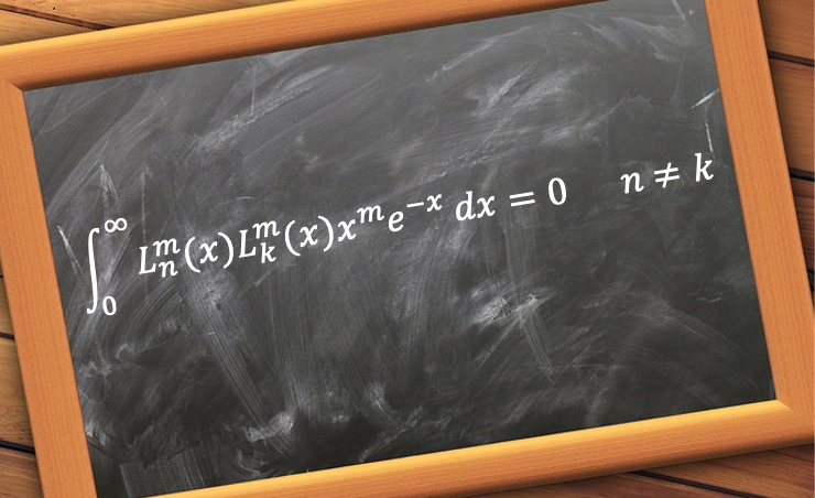
^{2l+2}e^{-\frac{2r}{na_0}}L_{n-l-1}^{2l+1}\biggr\(\frac{2r}{na_0}\biggr\)L_{n-l-1}^{2l+1}\biggr\(\frac{2r}{na_0}\biggr\)\biggr\]dr=\frac{2n(n+l)!}{(n-l-1)!}\frac{na_0}{2^{2l+3}}\;\;\;\;\;467)
The expression for the normalisation of eq466 is \vert^2r^2dr=1) or equivalently
or equivalently
^{2l+2}e^{-\frac{2r}{na_0}}L_{n-l-1}^{2l+1}\biggr\(\frac{2r}{na_0}\biggr\)L_{n-l-1}^{2l+1}\biggr\(\frac{2r}{na_0}\biggr\)dr=1)
Substituting eq467 yields
!}{2n(n+l)!}\frac{2^{2l+3}}{na_0}}\;\;\;\;\;\;\;\;468)
Therefore, the normalised radial wavefunction is
=\sqrt{\frac{(n-l-1)!}{2n(n+l)!}\frac{2^{2l+3}}{na_0}}\frac{1}{r}\biggr\(\frac{r}{na_0}\biggr\)^{l+1}e^{-\frac{r}{na_0}}L_{n-l-1}^{2l+1}\biggr\(\frac{2r}{na_0}\biggr\))
which can be easily rearranged to eq458.