BB84 is a quantum key distribution protocol that is based on photon polarisation states. It was invented by Charles Bennett and Gilles Brassard in 1984. The protocol can be broken down into the following steps:
1) The sender transmits a raw key in the form of a string of photons via an optical fibre to the receiver. Each photon is randomly chosen by the sender to be polarised along one of four directions: i) -direction or
(
), ii)
-direction or
(
), iii) ⤢ (
), iv) ⤡ (
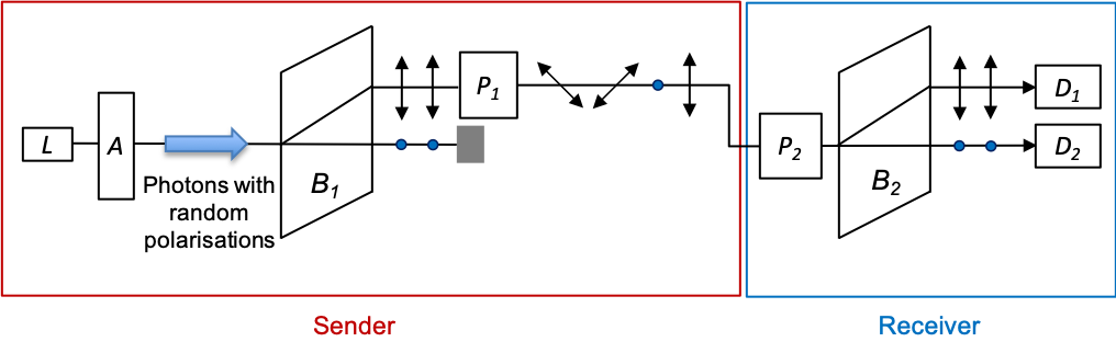
). This can be accomplished by passing photons generated by a laser
through an attenuator
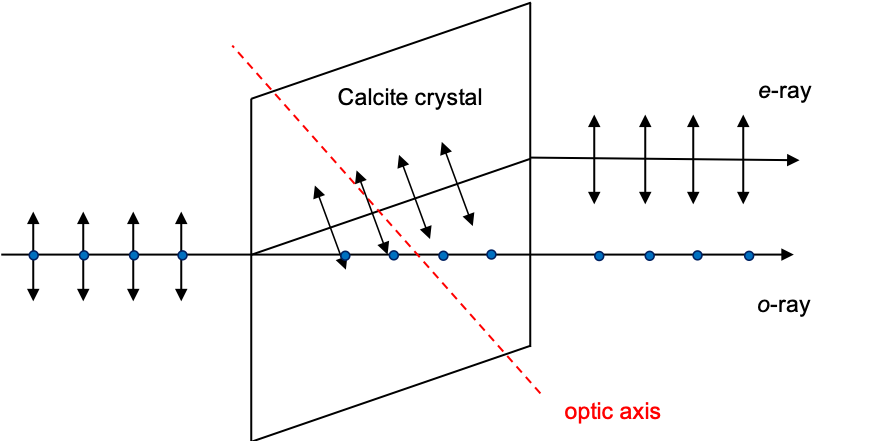
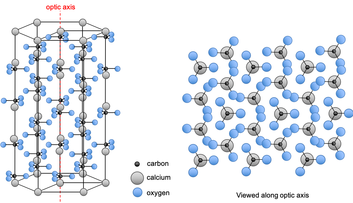
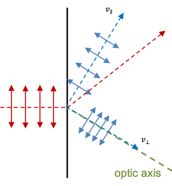
(a material that reduces the intensity of the laser beam through absorption or reflection to produce single photons), followed by a birefringent crystal
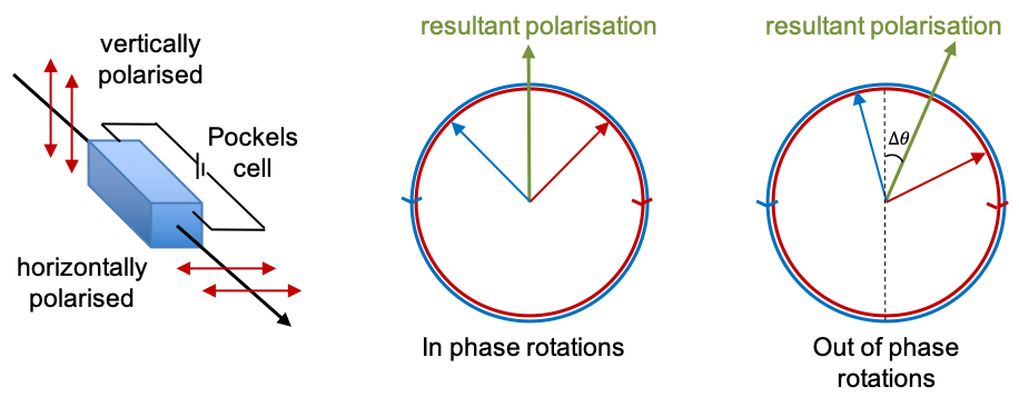
to separate photons into two orthogonal polarisations, one of which is passed through a Pockels cell
for the appropriate rotations (see diagram below).
2) The polarised photons are assigned the following qubit values: ,
, ⤢ = 0, ⤡ = 1, which can be grouped into the following bases:
| Basis | 0 | 1 |
| ⤢ | ⤡ |
3) The receiver, using Pockels cell , randomly selects one of two rotations (
representing the basis
, or
representing the basis
) to analyse each photon sent by the sender. The outputs of the detectors
and
are set to 1 and 0 respectively.
Assuming a raw key of twelve bits are sent, we may have the following case:
| Sender | Polarisation | ⤡ | ⤢ | ⤢ | ⤡ | ⤡ | |||||||
| Qubit value | 0 | 1 | 1 | 1 | 0 | 1 | 0 | 0 | 1 | 1 | 0 | 1 | |
| Receiver | Basis | ||||||||||||
| Qubit value | 0 | 1 | 1 | 0 | 0 | 0 | 0 | 0 | 1 | 1 | 1 | 1 | |
| Retained qubits | 0 | 1 | – | – | – | – | 0 | – | 1 | – | – | 1 | |
1) The sender and receiver share their bases with each other publicly (e.g. over the internet).
2) Only the qubits corresponding to polarisations with the same basis are retained. To complete the protocol, all other qubits can be converted to 0. The final key in the above example is 010000001001, which is used to encrypt a message (assuming of the same qubit-length) using modular addition.
Let’s suppose a third party intercepts the sender’s qubits and measures them using the same method as the receiver. The interceptor then has to guess the sender’s polarisation for each measured qubit and resend them to the receiver (see table below). Since the interceptor does not know the bases selected by the sender, the bits he measured are only useful if he is lucky enough to choose the same bases for the qubits that the sender and receiver eventually retained.
| Sender | Polarisation | ⤡ | ⤢ | ⤢ | ⤡ | ⤡ | |||||||
| Qubit value | 0 | 1 | 1 | 1 | 0 | 1 | 0 | 0 | 1 | 1 | 0 | 1 | |
| Interceptor | Basis | ||||||||||||
| Qubit value | 0 | 1 | 0 | 1 | 1 | 1 | 0 | 1 | 0 | 0 | 0 | 1 | |
| Resends | ⤢ | ⤢ | ⤡ | ⤡ | ⤢ | ⤡ | |||||||
| Receiver | Basis | ||||||||||||
| Qubit value | 1 | 1 | 0 | 0 | 1 | 0 | 0 | 1 | 0 | 0 | 0 | 1 | |
| Retained qubits | 1 | 1 | – | – | – | – | 0 | – | 0 | – | – | 1 | |
| Discrepancies | Y | N | – | – | – | – | N | – | Y | – | – | N | |
To detect the presence of an interceptor, the sender and receiver share pre-determined segments of qubits with each other. The probability that the sender and receiver select the same bases but the interceptor chooses different bases is , of which half the time the interceptor resend polarisations of the ‘wrong’ basis to the receiver. Therefore, the probability of the sender and the receiver detecting discrepancies in the retained qubits when they share segments of their qubit values is
(assuming the shared qubits are representative of a randomly selected segment), which is very significant if the qubit-length of the raw key is relatively long. For example, if the raw key has 72 qubits, of which 40 common qubits are eventually shared between the sender and the receiver, 5 retained qubits will be erroneous. When discrepancies are detected, the sender and receiver will discard the key and start over.