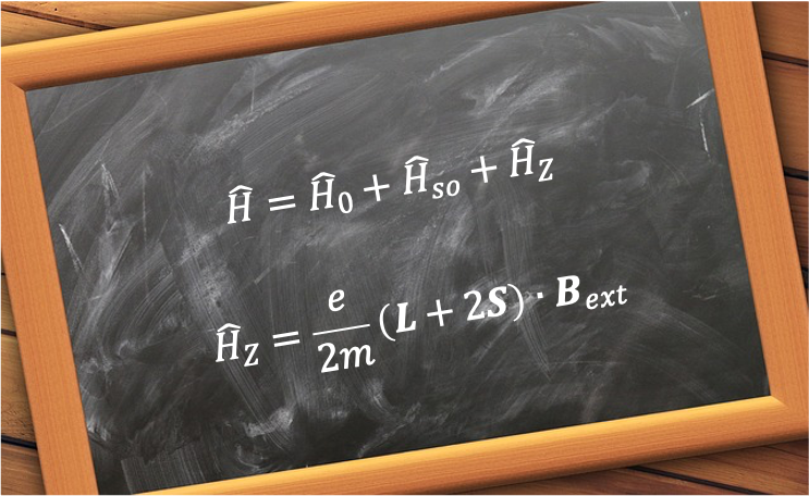
The intermediate-field case of the Zeeman effect is the regime in which an atom or molecule in an external static magnetic field exhibits splitting of its spectral lines into multiple components, with the field strength comparable to the internal spin–orbit interaction.
To analyse the intermediate-field regime, we consider a hydrogen atom in an external magnetic field whose strength is comparable to that of the internal spin-orbit coupling ( ). In this case, neither the coupled basis
  nor the uncoupled basis
  is strictly a good quantum state. Nevertheless, the Hamiltonian
  remains invariant under rotations about the direction of the external magnetic field (taken as the lab
  -axis).
With reference to eq330 and eq331, where the spin-orbit Hamiltonian is  , the perturbed part of the Hamiltonian becomes
)
if we take  , where
  is a unit vector.
The spin-orbit term  commutes with
  and
and  but not with
  or
or  , while the Zeeman term
 ) commutes with and , and hence with , but not with . Consequently,
commutes with and , and hence with , but not with . Consequently,  and
and  may still be regarded as a good quantum number.
Substituting +\hat{L}_z\hat{S}_z) into
into  gives:
+A\hat{L}_z\hat{S}_z+\frac{eB}{2m}(\hat{L}_z+2\hat{S}_z)\;\;\;\;\;\;\;\;340)
To determine the energy levels, we can no longer rely on the simple first-order perturbation formulas derived in eq334 or eq336. Instead, the spin-orbit Hamiltonian  and the Zeeman Hamiltonian
  must be treated on equal footing. One qualitative approach is to interpolate between the energy sublevels obtained in the weak-field and strong-field limits. However, a more rigorous method involves the following steps:
To illustrate this method, we consider the 2p1 configuration of the hydrogen atom, with  and
and  . In the absence of an external magnetic field, spin-orbit coupling (using LS coupling) splits the configuration into two energy levels,
  and
and  , with degeneracies
  and
and  respectively. Even though only
  remains a good quantum number, we can choose
  as the uncoupled basis state and form linear combinations to generate the eigenstates.
Since is the only conserved quantity, we group the eigenstates according to their values. For and , the possible values are  and
and  .
.
The basis states  and
and  corresponding to
  and
and  respectively are regarded as unmixed states because each value of corresponds to a unique pair of
  and
and  . Consequently, these states,
  and
and  , are eigenstates of the perturbed part of the Hamiltonian.
For  , there are two possible basis states,
  and
and  , and the corresponding eigenstates are linear combinations of these states:
  . Similarly, for
  , the eigenstates are linear combinations of
  and
and  , i.e.
  . We refer to these linear combinations as mixed states.
Having identified the eigenstates, the remaining task is to determine the energy levels. The expectation value for  is
is  , in which is given by eq340. From eq144, and noting that can be expressed as the Krönecker product
  ,
,
-m_l(m_l+1)}\vert l,m_l+1\rangle\otimes\hat{S}_-\vert s,m_s\rangle)
For , we have  . Similarly, using the spin analogue of eq144,
-m_l(m_l+1)}\vert s,m_s+1\rangle=0)
Furthermore,  and
and \vert m_l,m_s\rangle=\hbar(m_l+2m_s)\vert m_l,m_s\rangle) . Therefore,
. Therefore,

where  .
.
Using eq147 and its spin analogue, and repeating the above logic,

For the mixed state  , where
  and
and  , the Hamiltonian is:

Repeating the steps used for the unmixed states to compute the matrix elements gives:

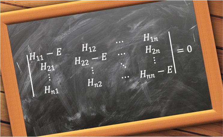
To find the eigenvalues, we solve the secular equation  or equivalently,

Expanding the determinant gives the characteristic equation:
E-\frac{A\hbar^2\mu_BB}{2}-\frac{A^2\hbar^4}{2}=0\;\;\;\;\;\;\;\;343)
Solving the quadratic equation yields two energy levels that depend on  :
:
\pm\sqrt{(\mu_BB)^2+A\hbar^2\mu_BB+\frac{9A^2\hbar^4}{4}}}{2}\;\;\;\;\;\;\;\;344)
A similar analysis for  , where
  and
and  leads to:

with
E+\frac{A\hbar^2\mu_BB}{2}-\frac{A^2\hbar^4}{2}=0\;\;\;\;\;\;\;\;345)
and
\pm\sqrt{(\mu_BB)^2-A\hbar^2\mu_BB+\frac{9A^2\hbar^4}{4}}}{2}\;\;\;\;\;\;\;\;346)
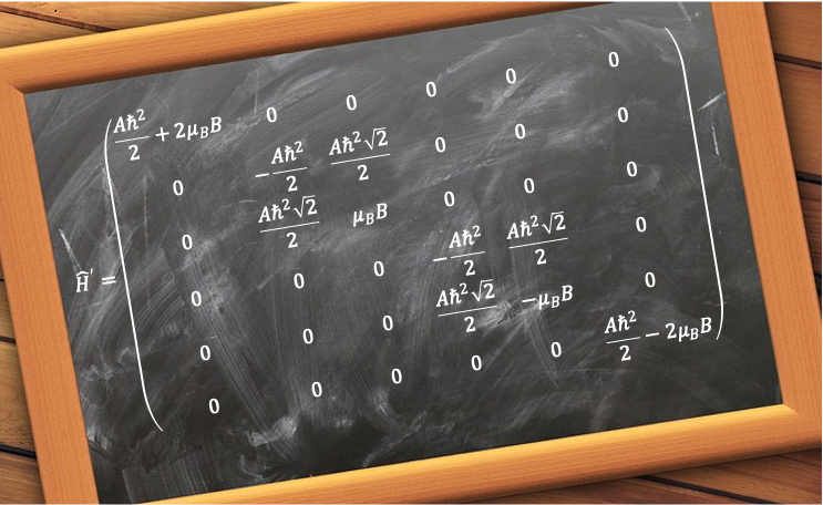
Therefore, the intermediate-field case results in six energy levels for the 2p1 configuration of the hydrogen atom, consistent with the weak-field and strong-field cases, with the perturbed portion of the Hamiltonian given by a  matrix:

To show that the matrix elements of are consistent with the eigenvalues at the extreme limits of , we consider the cases  and
and  .
.
When eq343 and eq345 reduce to the same equation:  , with solutions
  and
and  . These correspond to the spin-orbit energy levels and in the absence of an external magnetic field. Similarly, the eigenvalues of the unmixed states collapse onto the same energy as the level, namely
  . In other words, the degeneracies are restored, with being four-fold degenerate and being two-fold degenerate.
In the opposite limit , the unmixed-state eigenvalues become  , which agrees with the strong-field regime for the states
 =(\pm 1,\pm 1/2)) . For the mixed states, we refer to eq346, where the
. For the mixed states, we refer to eq346, where the ^2) and
and  terms dominate the discriminant, allowing it to be approximated by the perfect square
 ^2) . So,
. So,
\pm\biggr\(\mu_BB+\frac{A\hbar^2}{2}\biggr\)}{2}=\biggr\{\begin{matrix}\mu_BB\\-\frac{A\hbar^2}{2}\end{matrix}\;\;\;\;\;\;\;\;347)
Similarly, eq346 yields
\pm\biggr\(\mu_BB-\frac{A\hbar^2}{2}\biggr\)}{2}=\biggr\{\begin{matrix}-\frac{A\hbar^2}{2}\\-\mu_BB\end{matrix}\;\;\;\;\;\;\;\;348)
The energies given by eq347 and eq348 are again consistent with those obtained in the strong-field case.

Question
Why is the intermediate-field case of the Zeeman effect analysed using degenerate perturbation theory, while the weak-field and strong-field cases are not?
Answer
Degenerate perturbation theory can be applied to all three cases. However, in the weak-field and strong-field regimes the eigenvalues are usually obtained more simply by computing expectation values, since the relevant Hamiltonians are already diagonal in the corresponding unmixed eigenstate bases.