The study of nuclear statistics plays a crucial role in understanding the rotational states of atomic nuclei, particularly in systems composed of identical particles, for example, homonuclear diatomic molecules.
![]()
Nuclear statistics dictate which rotational states are populated for molecules with identical nuclei. This effect arises due to a postulate of quantum mechanics, which states that the total wavefunction of a molecule must be either symmetric or antisymmetric with respect to the exchange of identical nuclei, depending on whether the nuclei are bosons or fermions. Such a statistical constraint directly influences the observed spectroscopic transitions.
To understand how nuclear statistics constrain rotational states, we refer to the total wavefunction for a rotating molecule, which can be approximated as a product of its component wavefunctions:
where
is the nuclear spin wavefunction
is the rotational wavefunction
is the vibrational wavefunction
is the electronic wavefunction
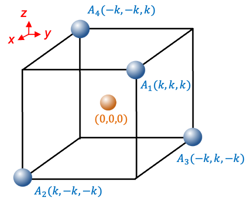
Consider the total ground state wavefunction of 16O2, where each nucleus is a boson. There are two unpaired electrons occupying separate degenerate antibonding molecular orbitals, while the remaining (core) electrons occupy doubly filled orbitals in singlet states.
The total two-electron wavefunction describing each doubly occupied molecular orbital (MO) is:
The spin wavefunction is antisymmetric under electron exchange. As required by the Pauli exclusion principle, the spatial component
must be symmetric with respect to electron exchange, and hence the form
. Under a nuclear exchange,
, which is independent of nuclear coordinates, is invariant. The spatial part
, being a product of two identical one-electron functions, also remains unchanged because any sign change on the individual orbital under a symmetry operation is cancelled out. Therefore,
is symmetric with respect to nuclear exchange.
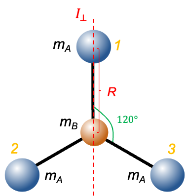
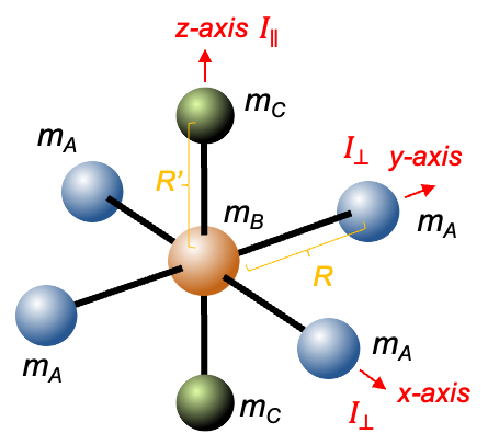
The molecular orbitals of the two unpaired electrons (triplet state) are formed from the atomic orbitals 2px and 2py of the oxygen atoms. Since the triplet spin wavefunction is symmetric under electron exchange, the associated spatial part of the wavefunction must be antisymmetric, in accordance with the Pauli exclusion principle:
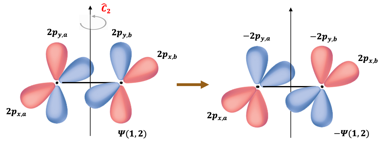
When subject to a rotation operation about the principal rotation axis perpendicular to the molecular
-axis (see above diagram),
It follows that the valence electronic wavefunction is antisymmetric with respect to this symmetry operation, which corresponds to nuclear exchange in the molecular frame. Therefore, the total ground state electronic wavefunction of 16O2, approximated as the product of the core and valence contributions, is antisymmetric under nuclear exchange.
With regard to eq97, the total vibrational ground state wavefunction of 16O2 is totally symmetric under all symmetry operations of the molecular point group, since these operations leave the squares of the normal coordinates invariant.
The nuclear spin wavefunction for 16O2 is given by (see this article for details), where each 16O nucleus has zero spin. Since both nuclear spin states are identical, i.e.
, swapping the subscripts results in the exact same wavefunction. Therefore, the nuclear spin wavefunction is symmetric under nuclear exchange.
Rotational wavefunctions are represented by spherical harmonics , where the symmetry under nuclear exchange depends on the value of
. These wavefunctions are symmetric for even
and antisymmetric for odd
, i.e. they change sign by
under an inversion. Since the total wavefunction of 16O2 must be symmetric, half of the possible rotational states are forbidden by nuclear statistics. In other words, 16O2 can only occupy odd rotational states in its ground electronic configuration.

Question
Prove that the rotational wavefunction of a diatomic molecule is symmetric for even and antisymmetric for odd
.
Answer
With reference to eq400, the unnormalised rotational wavefunction of a diatomic molecule is:
where .
The general and most comprehensive way to analyse the symmetry of a rotational wavefunction is to subject it to an inversion. In spherical coordinates, the inversion operator transforms a position vector from
to
, where the polar angle
is reflected about the equatorial plane and the azimuthal angle
is rotated by
. Since
, it follows that
Letting and using the chain rule
gives
, and hence
. Furthermore,
, where
. So,
. Therefore,
Since is always even, the wavefunction is symmetric with respect to inversion for even
and antisymmetric for odd
.
While nuclear statistics do not affect the value of the rotational energy levels, they can result in diminished spectral intensities or even “missing” peaks, particularly in Raman spectroscopy. However, this restriction does not apply to heteronuclear diatomic molecules, since the nuclei are not identical and there is no exchange symmetry requirement.
Question
How do nuclear statistics constrain rotational energy levels of ground state symmetrical linear polyatomic molecules like CO2?
Answer
The principles for analysing nuclear spin statistics in CO2 are similar to those for O2. ,
and
must be symmetric under nuclear exchange, which involves two oxygen nuclei in a closed-shell molecule. The ground state vibrational wavefunction of CO2 is also given by eq97, which is symmetric under nuclear exchange. Therefore, CO2 can only occupy even rotational states in its ground electronic and vibrational configuration.