Intermediate Chemistry - Mono Mole

April 30, 2024September 13, 2024

The Beer-Lambert law

The Beer-Lambert Law states that the absorbance of a solution is directly proportional to the path length of the sample and the concentration of the absorbing species in the solution.

Consider a beam of electromagnetic radiation with a narrow range of wavelengths $d\lambda$ passing through a sample of molar concentration $c$ and length $L$ . Let $N$ be the number of photons striking on the sample per unit time, and $dN$ be the number of photons absorbed by the sample. The probability of the number of photons absorbed by the sample ${\frac{dN}{N}}$ is dependent on the length of sample $dl$ and the concentration of the sample. Therefore, we have

$\frac{dN}{N}=kcdl$

where $k$ is a proportionality constant.

As spectroscopy involves the absorption of radiation intensity at different wavelengths, we need to express the above equation in terms of intensity.

The intensity of the radiation is proportional to the number of photons $N$ striking per unit area of the sample per unit time. Let the intensity of radiation that is incident on the sample and the outgoing intensity of the radiation be $I_0$ and $I$ respectively. It follows that, the greater the number of incident photons, the higher the outgoing intensity will be, i.e. $I\propto N$ . Furthermore, if $dI$ is the change in intensity after the radiation passes through the sample, then $dI\propto -dN$ , which implies that ${\frac{dI}{I}\propto -\frac{dN}{N}}$ . So, we have

$\frac{dI}{I}=-k'cdl$

where $k'$ is another proportionality constant.

Integrating the above equation throughout the length of the sample, we have $\int_{I_0}^{I}\frac{dI}{I}=-k'c\int_0^ldl$ , which gives $2.303log\frac{I}{I_0}=-k'lc$ or equivalently,

$A=\varepsilon lc\;\;\;\;\;\;\;\;1$

where $A=log\frac{I_0}{I}$ and $\varepsilon=\frac{k'}{2.303}$ .

Eq1 is the Beer-Lambert law. $A$ is the sample’s absorbance and $\varepsilon$ is known as the molar absorption coefficient, which represents the nature of the sample. Conventionally, the units of $c$ and $l$ are ${mol\;dm^{-3}}$ and $cm$ respectively. Moreover, $\varepsilon$ is expressed in ${dm^3mol^{-1}cm^{-1}}$ , and so, $A$ is unitless. The Beer-Lambert law is applicable to UV, visible and IR spectroscopy.

Next article: UV and visible spectroscopy

Previous article: Introduction to spectroscopy

Content page of UV-vis and IR spectroscopy

Content page of intermediate chemistry

April 30, 2024January 13, 2026

Introduction to spectroscopy

Spectroscopy is the scientific study of the absorption and emission of electromagnetic radiation by matter.

The instrument used for analysing these interactions is known as a spectrometer. A typical spectrometer consists of a light source that produces a beam with a range of electromagnetic frequencies (see diagram below). This beam passes through the sample, where it may be absorbed. The remaining transmitted radiation is detected and recorded, forming an absorption spectrum.

The absorption of a photon of energy $h\nu$ causes a chemical species to undergo a transition from a lower energy state $E_m$ to a higher energy state $E_n$ . Different magnitudes of $h\nu$ elicit various transitions. These transitions can occur between rotational states, vibrational states, electronic states, and even nuclear spin states of a chemical species (see diagram below).

A variety of spectroscopic methods are used to analyse these transitions. For example, infrared (IR) spectroscopy focuses on transitions between vibrational states, rotational spectroscopy analyses transitions between rotational states, Raman spectroscopy also studies transitions between both vibrational and rotational states, and nuclear magnetic resonance (NMR) spectroscopy studies transitions between different nuclear spin states.

Next article: The Beer-Lambert Law

Content page of UV-vis and IR spectroscopy

Content page of intermediate chemistry

January 25, 2023June 27, 2025

Derivation of the root mean square speed of a gas

The root mean square speed of a gas provides a measure of the average molecular speed in the gas.

Consider a gas particle of mass $m$ moving in a container to the right with velocity $v$ (see diagram below). The change in momentum of the particle $\Delta p$ in the $x$ -coordinate before and after colliding elastically with a surface of the container is

$\Delta p=-mv_x-mv_x=-2mv_x\;\;\;\;\;\;\;\;(1)$

with the particle colliding the same surface every

$\Delta t=\frac{dist}{speed}=\frac{2L}{\vert v_x\vert}\;\;\;\;\;\;\;\;(2)$

The force $F$ acting on the particle at collision is

$F=m\frac{\Delta v}{\Delta t}=\frac{\Delta p}{\Delta t}=-\frac{mv_x^2}{L}\;\;\;\;\;\;\;\;(3)$

By Newton’s third law, the force acting on the surface of the container by the particle is

$F=\frac{mv_x^2}{L}\;\;\;\;\;\;\;\;(4)$

The total force $F_T$ exerted on the surface by $N$ particles is

$F_T=\frac{mv_{x,1}^2}{L}+\frac{mv_{x,2}^2}{L}+\cdots+\frac{mv_{x,N}^2}{L}=\frac{Nm\overline{v_x^2}}{L}\;\;\;\;\;\;\;\;(5)$

where $\overline{v_x^2}=\frac{v_{x,1}^2+v_{x,2}^2+\cdots+v_{x,N}^2}{N}$ .

Comparing $\overline{v_x^2}$ and the definition of root mean square speed, we have $\overline{v_x^2}=v_{x,rms}^2$ , i.e. the square of the root mean square speed of the gas in the $x$ -direction.

If the container is three-dimensional (see above diagram), the velocity vector for a particle in Cartesian coordinates in three dimensions is:

$v^2=v_x^2+v_y^2+v_z^2\;\;\;\;\;\;\;\;(6)$

Even though a particle has three velocity components in space, the force exerted on the shaded wall is dependent only on the $x$ -component velocity of the particle.

To express the root mean square speed for $N$ particles, let’s begin by summing the squares of the velocity vectors of all particles:

$v_1^2+v_2^2+\cdots+v_N^2=(v_{x,1}^2+v_{y,1}^2+\cdots+v_{z,1}^2)+(v_{x,2}^2+v_{y,2}^2+\cdots+v_{z,2}^2)+\cdots+(v_{x,N}^2+v_{y,N}^2+\cdots+v_{z,N}^2)$

Next, group the velocity components and divide the equation throughout by $N$ ,

$\frac{v_1^2+v_2^2+\cdots+v_N^2}{N}=\frac{(v_{x,1}^2+v_{x,2}^2+\cdots+v_{x,N}^2)}{N}+\frac{(v_{y,1}^2+v_{y,2}^2+\cdots+v_{y,N}^2)}{N}+\cdots+\frac{(v_{z,1}^2+v_{z,2}^2+\cdots+v_{z,N}^2)}{N}$

$\overline{v^2}=\overline{v_x^2}+\overline{v_y^2}+\overline{v_z^2}\;\;\;\;\;\;\;\;(7)$

The velocity components of the particles in the container are assumed to be random, with the particles evenly distributed in the container at any time. $v_x$ , like $v_y$ and $v_z$ , can be positive or negative, but their squares, $v_x^2$ , $v_y^2$ and $v_z^2$ , are always positive. If the velocity components of the particles in the container are random, and the number of particles is very large,

$\overline{v_x^2}=\overline{v_y^2}=\overline{v_z^2}\;\;\;\;\;\;\;\;(8)$

Otherwise, there is a preference of direction in a particular axis and the particles’ movement is no longer random (you can convince yourself the validity of eq8 by summing the squares of three sets of randomly generated numbers in a spreadsheet and finding their averages; the larger the number of elements in each set, the closer the average values are to each other). Hence, we can rewrite eq7 as:

$\overline{v^2}=3\overline{v_x^2}\;\;\;\;\;\;\;\;(9)$

Substituting eq9 in eq5 gives

$F_T=\frac{Nm\overline{v^2}}{3L}\;\;\;\;\;\;\;\;(10)$

The pressure $p$ (not to be confused with momentum) exerted by $N$ particles on the shaded wall is

$p=\frac{F_T}{A}=\frac{Nm\overline{v^2}}{3V}$

where $V$ is the volume of the container.

Hence,

$pV=\frac{1}{3}Nm\overline{v^2}=\frac{2}{3}N\left(\frac{1}{2}m\overline{v^2}\right)\;\;\;\;\;\;\;\;(11)$

Substituting the ideal gas law in eq11 yields

$nRT=\frac{1}{3}Nm\overline{v^2}=\frac{2}{3}N\left(\frac{1}{2}m\overline{v^2}\right)\;\;\;\;\;\;\;\;(11)$

Since $R=N_Ak$ (see this article for derivation ) and $N=nN_A$ ,

$nkT=\frac{2}{3}n\left(\frac{1}{2}m\overline{v^2}\right)$

$\frac{3}{2}kT=\frac{1}{2}m\overline{v^2}=\langle KE\rangle\;\;\;\;\;\;\;\;(12)$

Since $\overline{v^2}=\frac{v_1^2+v_2^2+\cdots+v_N^2}{N}$ and the root mean square speed is $v_{rms}=\sqrt{\frac{v_1^2+v_2^2+\cdots+v_N^2}{N}}$ , we have $\overline{v^2}=v_{rms}^2$ . Therefore,

$v_{rms}=\sqrt{\frac{3kT}{m}}\;\;\;\;or\;\;\;\;v_{rms}=\sqrt{\frac{3RT}{M}}\;\;\;\;\;\;\;\;(13)$

where $M$ is the molar mass of the gas.

Previous article: Root mean square speed of a gas

Content page of kinetic theory of gases

Content page of intermediate chemistry

Main content page

January 25, 2023September 25, 2024

Root mean square speed of a gas

The root mean square speed of a gas is a statistical measure of the average speed of each particle in the gas.

As mentioned in an earlier article, a gas in a container is made up of point masses that are moving randomly and colliding elastically with each other. The velocity of a gas particle is a vector with both magnitude and direction. With every elastic collision, the magnitude of a gas particle’s velocity is unchanged but its direction changes. The particles remain evenly distributed because the sum of the velocity vectors of all particles in the container at any time is zero (a non-zero net velocity implies that the particles are moving in a particular direction and are no longer in random motion).

We cannot determine the individual velocity of a gas particle and have to rely on an average value, which is zero as explained above. This poses a problem and we need to devise a different way to average the velocities of the particles. This new averaging method, which is described in the previous article, is called the root mean square speed and is given by

$v_{rms}=\sqrt{\frac{v_1^2+v_2^2+\cdots+v_N^2}{N}}$

In the ideal case where the magnitudes of the velocities of all the particles are the same, $v_{rms}$ is the same as taking the average of the absolute values of the velocities of the particles.

Previous article: Standard deviation

Next article: Derivation of the root mean square speed of a gas

Content page of kinetic theory of gases

Content page of intermediate chemistry

Main content page

January 25, 2023September 25, 2024

Standard deviation

The standard deviation of a set of numbers is the measure of the dispersion of the numbers with respect to the mean.

Consider the following sets of numbers:

-2, -2, 2, 2 with a mean of 0

-3, -1, 0, 4 with a mean of 0

The two sets of numbers have the same mean, $\mu$ , or average value. However, the numbers in the first set are clearly less dispersed from the central value of 0 than those in the second set. Therefore, we need an averaging indicator that can tell us the deviation or spread of the numbers about the mean. Suppose we find the average of the absolute values of the numbers:

$\frac{\vert-2\vert+\vert-2\vert+\vert2\vert+\vert2\vert}{4}=2$

$\frac{\vert-3\vert+\vert-1\vert+\vert0\vert+\vert4\vert}{4}=2$

We end up with the same value with no information regarding the respective spreads. If we try this approach,

$\sqrt{\frac{(-2-0)^2+(-2-0)^2+(2-0)^2+(2-0)^2}{4}}=2$

$\sqrt{\frac{(-3-0)^2+(-1-0)^2+(0-0)^2+(4-0)^2}{4}}\approx2.55$

we have a reasonable distinction between the spreads.

What we have done for each set in the above computation is that we have:

Taken the difference between an element in the set and the mean.
Squared the difference and repeat step 1 and step 2 for the rest of the elements in the set.
Summed all the squared differences.
Divided the sum with the number of elements in the set.
Computed the square root of the result in step 4.

This method of measure is called standard deviation $\sigma$ . In general,

$\sigma=\sqrt{\frac{(x_1-\mu)^2+(x_2-\mu)^2+\cdots+(x_N-\mu)^2}{N}}$

If the mean of the set of numbers is zero,

$\sigma_{rms}=\sqrt{\frac{x_1^2+x_2^2+\cdots+x_N^2}{N}}$

We call the standard deviation for this special case, the root mean square value of the set. Notice that the results obtained from the absolute value method and the standard deviation method (or root mean square) are the same if the magnitudes of all the elements in the set are the same.

Previous article: Kinetic theory of gases (overview)

Next article: Root mean square speed of a gas

Content page of kinetic theory of gases

Content page of intermediate chemistry

Main content page

January 25, 2023September 14, 2025

Kinetic theory of gases (overview)

The kinetic theory of gases describes the macroscopic properties of gases by analysing gaseous behaviour at the molecular level.

The theory assumes that a gas is composed of point masses moving randomly with different velocities in straight lines within a container. As they move, they may collide elastically with each other or with the walls of the container. The first important concept of the kinetic theory of gases is the root mean square speed of a gas.

Next article: Standard deviation

Content page of kinetic theory of gases

Content page of intermediate chemistry

Main content page

November 24, 2019September 25, 2024

Spin-spin coupling (nuclear-magnetic resonance)

Spin-spin coupling in nuclear magnetic resonance spectroscopy refers to the magnetic interactions between neighbouring nuclei that are not equivalent, leading to a change in resonance frequencies of the nuclei. As mentioned in an earlier article, the nucleus of an atom possesses a magnetic moment that generates a small magnetic field. If two NMR-active atoms (I ≠ 0) are in vicinity of each other, e.g. protons in the moiety HC-CH, the magnetic field of one ¹H can shield or deshield the magnetic field of the other ¹H, thereby slightly changing its shielding constant and therefore changing its resonance frequency.

In general, we refer to the following rules to determine the extent of nuclear spin-spin coupling:

1. Spin-spin coupling occurs in all NMR-active nuclei. However, the coupling between two or more equivalent nuclei results in the same resonance energy of transition and therefore has no effect on the chemical shifts of the nuclei.
2. Spin-spin coupling is negligible between nuclei separated by four or more bonds, e.g. the protons in HC-CH are separated by 3 bonds and consequently display coupling effects.
3. The changes in chemical shifts of spin-coupled nuclei are usually much smaller than the difference in chemical shifts between the nuclei.

The effects of spin-spin coupling are visible on a high resolution NMR spectrum. An example is the spectrum of ethanol, CH₃CH₂OH:

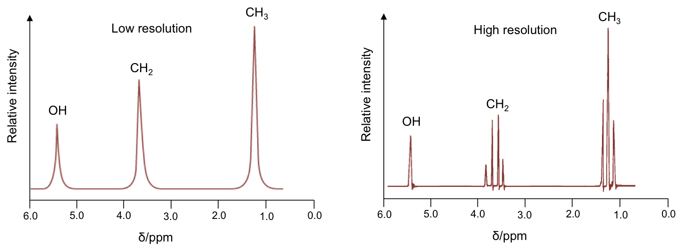
Effects of spin-spin coupling on CH₃ protons

According to rule 1, the three¹Hs in the CH₃ moiety are equivalent and spin-couple one another without affecting the position and shape of the CH₃ peak in the spectrum. However, they are not equivalent to the two protons in CH₂, which have the following possible spin orientations:

The percentages represent the statistical occurrences of the paired orientations in a sample of ethanol molecules, with M_I= Σm_I, i.e. the total nuclear spin magnetic number. Depending on the spin orientation of a proton in the CH₃ moiety, the paired orientations of M_I= +1 or M_I= -1 of protons in CH₂ either shield or deshield that proton, while the paired orientations of M_I= 0 in CH₂ does not affect the proton’s magnetic field. The result is a splitting of the single CH₃ peak into a triplet, with the middle peak retaining the same chemical shift as CH₃ without spin-spin coupling effect, and an equal up and down shift for the left and right peaks. The relative intensity of the left:middle:right peaks is 1:2:1 (see high resolution diagram above).

CH₃ protons are separated from the hydroxyl ¹H by four bonds. So, according to rule 2, any coupling effect is negligible.

Effects of spin-spin coupling on CH₂ protons

Using the same logic, the possible spin orientations of the three¹Hs in the CH₃ moiety are:

The four M_Ivalues split the single CH₂ peak into a quartet, with the distribution of four peaks along a vertical line of reflection that intersects the original chemical shift of CH₂ without spin-spin coupling effect. The relative intensity of the peaks is 1:3:3:1 (see high resolution diagram above).

Question

Why is the OH peak not a triplet and why is there no coupling effect between the hydroxyl ¹H and the CH₂ protons?

Answer

The presence of H₃O⁺ or OH^– in the sample, even in minute amounts, catalyses the exchange of hydroxyl protons between ethanol molecules. This exchange is fast enough to negate the spin-spin coupling effect between the hydroxyl proton and the CH₂ protons. The hydroxyl protons can also be swapped with protons from H₃O⁺, which is why the OH peak may disappear when D₂O is added to the ethanol sample (I_D= 0).

Finally, in cases where rule 3 fails, i.e. the changes in chemical shifts of spin-coupled nuclei are comparable to the difference in chemical shifts between the nuclei, the spectrum can become complex.

Question

Why are all peaks in a ¹³C NMR spectrum singlets?

Answer

¹³C, like ¹H, has a nuclear spin of I= ½ and is expected to experience spin-spin coupling with neighbouring ¹³C and ¹H nuclei. The natural abundance of ¹³C is only 1.1% and therefore the probability of a molecule having ¹³C adjacent nuclides is almost zero. However, ¹³C–¹H spin-spin coupling is ubiquitous. To avoid a complicated ¹³C spectrum, a technique called proton decoupling is used, where protons of molecules in a sample are irradiated with a secondary radiofrequency wave. The protons undergo rapid spin reorientations that result in their net M_I being zero.

Question

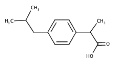
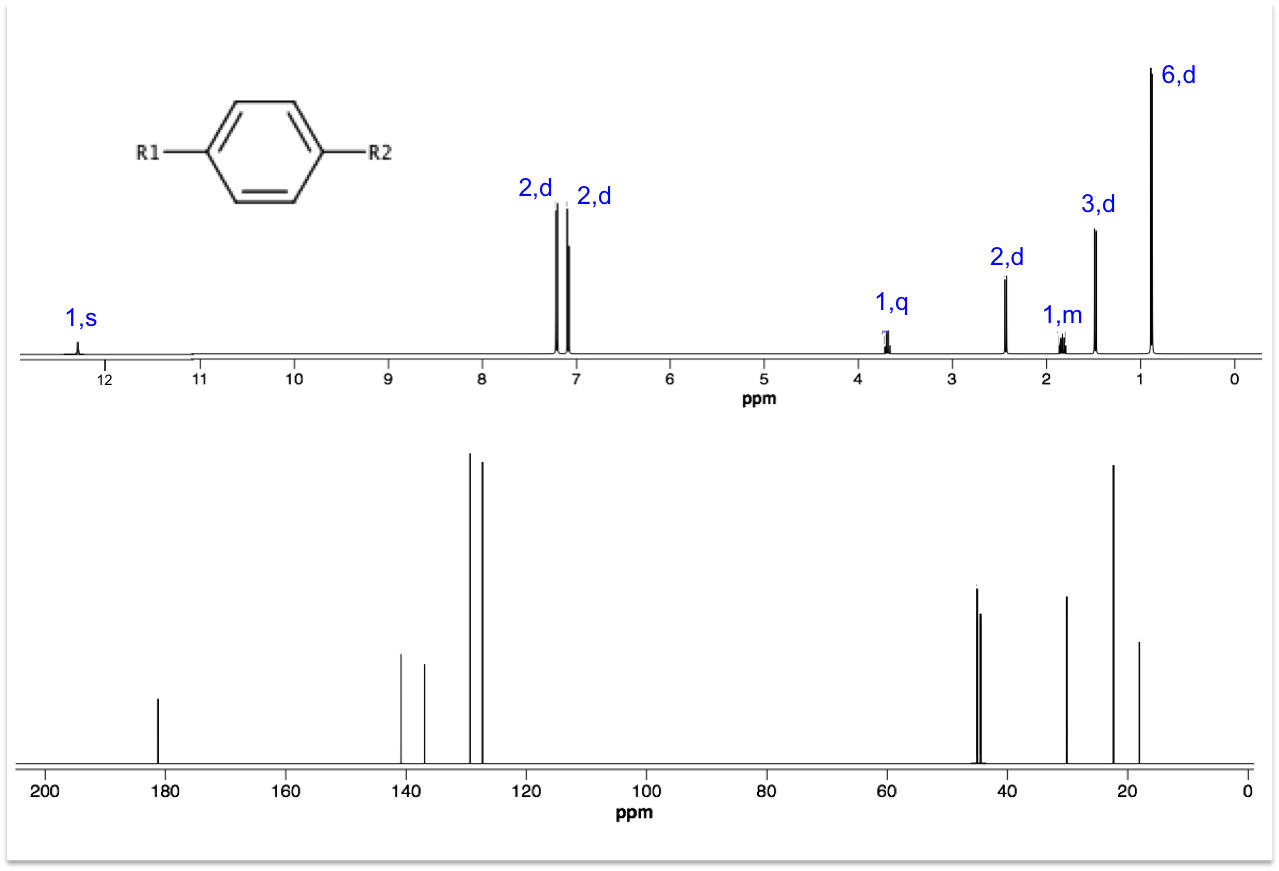
Deduce the structures for R1 and R2 using the ¹H and ¹³C spectra below. Hint: Ar–¹³C 45 ppm.

Answer

Even though ¹³C peak areas are not a reliable indicator of the relative number of carbons, we can make a guess of the carbon numbers by comparing the peak heights. Let’s assume the three taller peaks represent two carbons each, which gives a total of 13 carbons in the molecule.

The peak at 0.90 ppm of the top spectrum is a doublet of 6 protons, which suggests an isopropyl group. The doublet of 3 protons at 1.50 ppm is mostly likely a methyl group. The singlet at 12.34 ppm is characteristic of a carboxyl proton. A pair of doublets at 7.08-7.22 ppm, each with two protons, refers to protons on the benzene ring. That leaves us with 2 carbons associated with the quartet at 3.69 ppm and the doublet at 2.45 ppm. These two carbons have almost the same chemical shift of 45 ppm in the ¹³C spectrum, which according to the hint are carbons adjacent to the benzene ring. Putting everything together, we have the following structure (ibuprofen):

Previous article: Chemical shift

Content page of nuclear magnetic resonance

Content page of intermediate chemistry

Main content page

November 24, 2019March 14, 2026

Chemical shift (nuclear magnetic resonance)

The chemical shift δ in nuclear magnetic resonance spectroscopy is a measure of the spin transition frequency of a nuclide with respect to a standard nuclide. It is dependent on the identity of the nuclide and the chemical environment of the nuclide. From the previous article, we learned that the concept of nuclear magnetic resonance involves analysing resonance signals of nuclides by varying an alternating electromagnetic frequency v at a constant external magnetic field B, or by varying an alternating B at a constant v. According to Lenz’s law, a changing B induces an opposite magnetic field in an electron-filled system like an atom. The magnitude of the induced magnetic field is dependent on the atom’s electron density, which is influenced by neighbouring atoms. Since this induced magnetic field is directionally opposite to the external magnetic field, the effective external magnetic field felt by the nucleus is:

$B_{eff}=B-\sigma B\; \; \; \; \; \; \; \; 3$

where σ is a constant called the shielding constant, which varies according to the chemical environment of an atom.

For example, ¹H in the aldehyde functional group RCHO experiences a larger B_eff than ¹H in CH₄. This is because the electropositive carbonyl carbon reduces the electron density around the hydrogen nucleus (deshield), resulting in a lower induced magnetic field when the ¹H nucleus is exposed to an external magnetic field. We say that the shielding constant of ¹H in the aldehyde functional group of RCHO is smaller than that of ¹H in CH₄, or that ¹H in the aldehyde functional group of RCHO is relatively more deshielded than ¹H in CH₄(note that all ¹Hs in CH₄ are chemically equivalent).

Substituting eq3 and the Planck relation in eq2 of a previous article, we have

$v=\frac{\gamma B}{2\pi}\left ( 1-\sigma \right )\; \; \; \; \; \; \; \; 4$

Eq4 shows that if B is fixed (or if v is fixed), the radiofrequency v (or the external magnetic field B) needed to stimulate a nuclear spin transition is dependent on the gyromagnetic ratio $\gamma$ of the nuclide and the shielding constant. The remaining task is to set up a convenient measure, i.e. a scale, to represent the resonance frequencies for different nuclides. This scale, known as the chemical shift δ, is:

$\delta=\frac{v-v^o}{v^o}\times 10^6\; \; \; \; \; \; \; \; 5$

where v^o is the resonance frequency of a reference nuclide — tetramethylsilane (TMS) with the molecular formula Si(CH₃)₄ is commonly used as a reference in ¹H-NMR.

The reason why the fractional change term is multiplied by 10⁶ is that the numerator is expressed in hertz, while the denominator is in megahertz. For example, the resonance frequency of ¹H in TMS at a particular fixed B is 300 MHz, and that the resonance frequency of a ¹H in a sample that we are investigating is 300.0003 MHz at the same B. We would expect 2 peaks in the NMR spectrum, one for the chemically equivalent ¹Hs in TMS at δ = 0 (substituting v = v^o in eq5), and the second peak for ¹H-sample at:

$\delta=\frac{300\, Hz}{300\, MHz}\times10^6=1$

Since $\frac{Hz}{MHz}$ is 1 part per million, the units for δ is ppm. Therefore, instead of plotting the horizontal axis of the NMR spectrum in Hz or MHz, we plot it in δ, which has a simpler value. A typical low-resolution spectrum looks like this:

The horizontal axis is plotted such that the more heavily shielded nuclei appear to the right of the spectrum. The small peak at 0.0 ppm corresponds to ¹H from TMS. The areas under the peaks reflect the relative number of chemically equivalent ¹H for the respective chemical shift.

Some common chemical shifts of ¹H nuclides are as follows:

¹H nuclides	δ/ ppm
TMS	0.0
RCH₃	0.7 – 1.2
RCH₂R	1.1 – 1.5
R₃CH	1.6 – 2.0
ArCH₃, ArCH₂R, ArCHR₂	2.3 – 2.7
CH₃COR	2.0 – 3.0
-OCH₃, -OCH₂R, -OCHR₂	3.0 – 4.0
R_aCH_bX where a = 0,1,2 b = 1,2,3 X = Cl, Br	3.0 – 4.2
RNH₂	1.0 – 4.8
ROH	1.0 – 6.0
ArH	6.5 – 9.0
RCHO	9.5 – 10.5
RCO₂H	10.0 – 13.0

¹³C also has a nuclear spin of ½ and is NMR active. However, a large sample is needed for analysis, as its natural abundance is about 1.1%. The typical resonance frequency of a ¹³C nuclide is a quarter of that of a ¹H nuclide, which allows ¹³C spectra to be generated separately from ¹H spectra. The chemical shift of ¹³C ranges from 0 ppm to 220 ppm. Unlike a ¹H spectrum, the areas under peaks in a ¹³C spectrum are not a reliable indication of the relative number of carbons. This is because some carbon signals, e.g. carbonyl carbons, are weaker than other carbon signals, e.g. methyl carbons.

Question

Do the protons on the marked carbon have the same chemical shift?

Answer

The two protons, H_a and H_b, have different chemical shifts, as they are not equivalent (see the Newman projection below):

Next article: Spin-spin coupling

Previous article: Instrumentation

Content page of nuclear magnetic resonance

Content page of intermediate chemistry

Main content page

November 24, 2019July 24, 2025

Instrumentation (nuclear magnetic resonance)

A simple version of a nuclear magnetic resonance (NMR) spectrometer consists of the following:

1. A strong magnet to provide a uniform magnetic field B (e.g. 2.35 T) to split the energy levels of nuclides in a sample.
2. The sample in a glass tube that is rotated to allow uniform exposure to B.
3. A coil (blue lines) connected to a radiofrequency transmitter with a varying AC voltage. The AC voltage is gradually increased during the experiment to generate electromagnetic waves of increasing frequencies.
4. A coil wound round the sample tube and connected to a radiofrequency detector. The flipping of nuclear spins, when nuclides are excited at the appropriate electromagnetic frequencies, results in a change in magnetic dipole moment of the nuclides. This change in magnetic dipole moment induces a current in this coil, which is recorded and analysed by a computer.

Such an NMR spectrometer design, where the external magnetic field strength B is fixed while the electromagnetic radiation frequency v is varied, is called a continuous wave NMR (CW-NMR). An alternate design of a CW-NMR has a varying B and a constant v. In this design, a varying-AC coil is wound round the magnet, while a second coil with a fixed AC voltage is wrapped round the sample tube. Measurements are made for the changes in impedance (resistance of an AC circuit) of the second coil when nuclear spin transitions occur. Finally, a more sophisticated NMR spectrometer design exposes the sample to a short and intense burst of radiofrequency radiation called an electromagnetic pulse, and subsequently analyses the data using the mathematical concept of Fourier transform.

Next article: Chemical shift

Previous article: Nuclear magnetic dipole moment in an external magnetic field

Content page of nuclear magnetic resonance

Content page of intermediate chemistry

Main content page

November 24, 2019September 25, 2024

Nuclear magnetic dipole moment in an external magnetic field

We have mentioned in a quantum chemistry article that the nucleus of an atom (e.g. ¹H and ¹³C) possesses an intrinsic angular momentum called spin I and therefore a magnetic dipole moment μ, which tends to align parallel to an external magnetic field B in two possible directions (see diagram below).

Like tiny magnets, we would expect all dipoles of a sample of nuclei to align in the direction of an external field to achieve a lower energy state. However, at room temperature, the dipoles are constantly exchanging between the two forms, to the extent that at equilibrium, there is a slight excess of nuclei with dipoles that are aligned in the direction of the field. This behaviour of nuclear magnetic dipole moments in the presence of an external magnetic field at room temperature splits the energy of nuclei E_N into two levels (see diagram below).

It is found that the energy gap between the two levels ΔE is proportional to the external magnetic field:

$\Delta E=\hbar \gamma B\; \; \; \; \; \; \; \; 1$

where $\hbar \gamma$ is proportionality constant, with $\gamma$ being the gyromagnetic ratio, whose value is dependent on the identity of the nucleus.

Due to the slight excess of nuclei at the lower level at room temperature when B > 0, a net upward spin transition occurs when the nuclei are excited with radiation corresponding to ΔE. As the gyromagnetic ratio is nuclide-specific, ΔE varies for different nuclide at a fixed value of B. Furthermore, the effective external magnetic field B_eff experienced by a nucleus is dependent on the magnetic environment of the nucleus, which changes eq1 to:

$\Delta E=\hbar \gamma B_{eff}\; \; \; \; \; \; \; \; 2$

Eq2 is the heart of the analytical technique of nuclear magnetic resonance, where the identity and location of an unknown nuclide is determined by exposing the nuclide to a constant magnetic field and subsequently detecting its transition frequency.

Question

What are the typical frequencies for nuclear spin transitions? Why are nuclei with I = 0 not NMR active?

Answer

The frequencies needed for nuclear spin transitions, called resonance frequencies, are in the radiofrequency range. For example, γ for ¹H that is exposed to an external magnetic field of 9.4 T is 26.75 x 10⁷ T^-1s^-1. Substituting these values and the Planck relation ΔE = hv in eq1, we have v = 400.2 MHz.

The formula for the change in energy of a nuclear magnetic dipole moment in the presence of a magnetic field is:

$E_\pm =-m_I\hbar \gamma B$

A nuclide with spin I = 0 is associated with the nuclear magnetic spin number of m_I = 0, resulting in $E_\pm$ = 0. However, a nuclide with spin I = ½ has the nuclear magnetic spin numbers of m_I = +½ and m_I = -½, which gives:

Next article: UV and visible spectroscopy

Previous article: Introduction to spectroscopy

Next article: The Beer-Lambert Law

Previous article: Root mean square speed of a gas

Previous article: Standard deviation

Next article: Derivation of the root mean square speed of a gas

Previous article: Kinetic theory of gases (overview)

Next article: Root mean square speed of a gas

Next article: Standard deviation

Question

Answer

Question

Answer

Question

Answer

Previous article: Chemical shift

Question

Answer

Next article: Spin-spin coupling

Previous article: Instrumentation

Next article: Chemical shift

Previous article: Nuclear magnetic dipole moment in an external magnetic field

Question

Answer

Next article: Instrumentation