d-orbital

A d-orbital, defined by the quantum number $l=2$ , is a region of space around the nucleus where an electron is most likely to be found. The letter ”d” is of spectroscopic origin, standing for ‘diffuse’.

One-electron d-orbital wavefunctions can be expressed using the total wavefunction of a hydrogenic atom:

$\psi=R_{n,l}(r)Y_l^{\vert m_l\vert}(\theta,\phi)$

where

$R_{n,l}(r)=N_{n,l}\frac{1}{r}\biggr$\frac{r}{na_0}\biggr$^{l+1}e^{-\frac{r}{na_0}}L_{n-l-1}^{2l+1}\biggr$\frac{2r}{na_0}\biggr$$ , the radial wavefunction, is the radial component of $\psi$ .
$Y_l^{\vert m_l\vert}(\theta,\phi)=N_l^{\vert m_l\vert}P_l^{\vert m_l\vert}(cos\theta)e^{im_l\phi}$ , the spherical harmonics, is the angular component of $\psi$ .
$L_{n-l-1}^{2l+1}=\sum_{k=0}^{n-l-1}(-1)^k\frac{(n+l)!}{k!(k+2l+1)!(n-l-1-k)!}\biggr$\frac{2r}{na_0}\biggr$^k$ are the associated Laguerre polynomials.
$P_l^{\vert m_l\vert}(cos\theta)=\frac{1}{2^ll!}(1-cos^2\theta)^{\frac{\vert m_l\vert}{2}}\frac{d^{l+\vert m_l\vert}}{dcos\theta^{l+\vert m_l\vert}}(cos^2\theta-1)^l$ are the associated Legendre polynomials.
$N_{n,l}=\sqrt{\frac{(n-l-1)!}{2n(n+l)!}\frac{2^{2l+3}}{na_0}}$ is the normalisation constant of the radial wavefunction.
$N_l^{\vert m_l\vert}=\frac{1}{\sqrt{2\pi}}\biggr\[\frac{2l+1}{2}\frac{(l-\vert m_l\vert)!}{(l+\vert m_l\vert)!}\biggr\]^{\frac{1}{2}}$ is the normalisation constant of the spherical harmonics.
$n$ is the principal quantum number, where $n=1,2,\cdots$
$l$ is the orbital angular momentum quantum number (also known as azimuthal quantum number), where $l=0,1,2,\cdots$ and $l\leq n-1$ .
$m_l$ is the magnetic quantum number, where $-l\leq m_l\leq l$ .

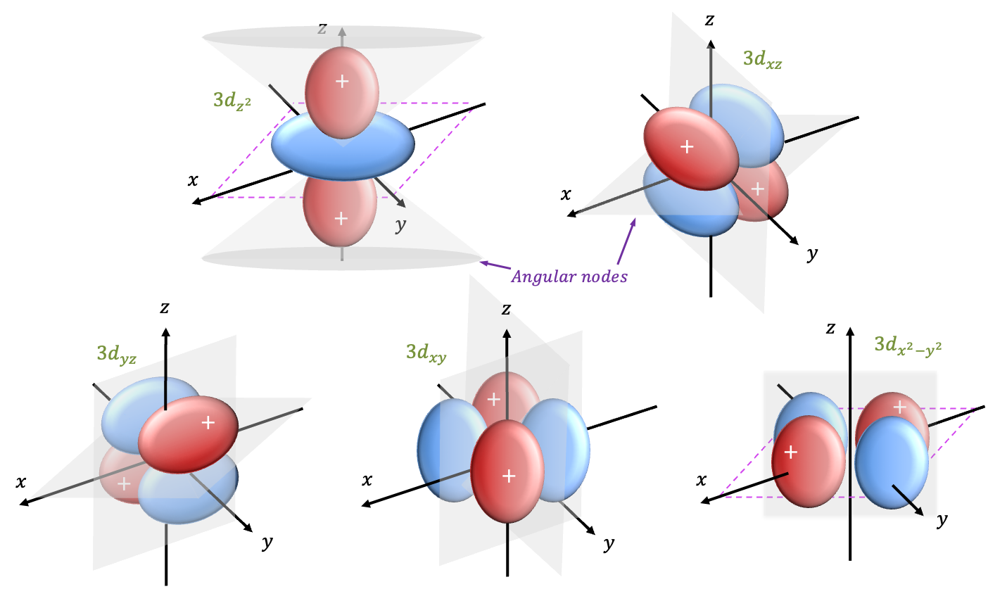
The principal quantum number, $n$ , is also called a shell. Since $-2\leq m_l\leq 2$ when $l=2$ , there are five d-orbitals that are characterised by the set of quantum numbers $\{n,l,m_l\}$ of $\{n,2,2\}$ , $\{n,2,1\}$ , $\{n,2,0\}$ , $\{n,2,-1\}$ and $\{n,2,-2\}$ in each shell for $n\geq 3$ . Four of the five d-orbitals have cloverleaf shapes, while the fifth has a lobular structure along the $z$ -axis with a doughnut-shaped region around the equatorial plane. Each of the five d-orbitals has two angular nodes. Consider the set $\{3,2,0\}$ . Substituting these values into the explicit formula for $R_{n,l}(r)Y_l^{\vert m_l\vert}(\theta,\phi)$ yields:

$R_{3,2}(r)Y_2^{0}(\theta,\phi)=r^2(3cos^2\theta-1)f(r)$

where $f(r)=\frac{1}{81\sqrt{6\pi}}\sqrt{\biggr$\frac{1}{a_0}\biggr$^7}e^{-\frac{r}{3a_0}}$ .

Converting from spherical coordinates to Cartesian coordinates, where $z=rcos\theta$ , gives

$\psi_{3d_{z^2}}=z^23f(r)-r^2f(r)\;\;\;\;\;\;\;\;478$

Eq478 is known as the wavefunction for the $3d_{z^2}$ orbital. When $z=\frac{r}{\sqrt{3}}$ or $z=-\frac{r}{\sqrt{3}}$ , $\psi_{3d_{z^2}}=0$ . Therefore, the wavefunction is zero at $\theta=arccos\biggr$\pm\frac{1}{\sqrt{3}}\biggr$$ in spherical coordinates. This implies that the angular nodes occur at two conical surfaces with their apices at the origin, extending at $\theta=arccos\biggr$\pm\frac{1}{\sqrt{3}}\biggr$$ along the $z$ -axis.

For the sets $\{3,2,1\}$ and $\{3,2,-1\}$ , we have ${\psi_{d_1}=\frac{1}{81\sqrt{\pi}}\sqrt{\biggr$\frac{1}{a_0}\biggr$^7}r^2e^{-\frac{r}{3a_0}}sin\theta cos\theta e^{i\phi}}$ and ${\psi_{d_{-1}}=\frac{1}{81\sqrt{\pi}}\sqrt{\biggr$\frac{1}{a_0}\biggr$^7}r^2e^{-\frac{r}{3a_0}}sin\theta cos\theta e^{-i\phi}}$ , respectively. These two wavefunctions include the factor $e^{\pm i\phi}$ , which may complicate calculations when they undergo symmetry operations. Therefore, we take linear combinations of these wavefunctions to form simpler wavefunctions. The first linear combination is ${\psi_{d_1}+\psi_{d_{-1}}=\frac{2}{81\sqrt{\pi}}\sqrt{\biggr$\frac{1}{a_0}\biggr$^7}r^2e^{-\frac{r}{3a_0}}sin\theta\cos\theta\cos\phi}$ , which normalises to ${\frac{1}{81}\sqrt{\frac{2}{\pi}\biggr$\frac{1}{a_0}\biggr$^7}r^2e^{-\frac{r}{3a_0}}sin\theta\cos\theta\cos\phi}$ , or equivalently in Cartesian coordinates:

$\psi_{3d_{xz}}=xzf(r)\;\;\;\;\;\;\;\;479$

where $f(r)=\frac{1}{81}\sqrt{\frac{2}{\pi}\biggr$\frac{1}{a_0}\biggr$^7}e^{-\frac{r}{3a_0}}$ and $x=rsin\theta cos\phi$ .

$\psi_{3d_{xz}}=0$ when $x=0$ or $z=0$ . This implies that $\psi_{3d_{xz}}$ has two nodal planes: $yz$ and $xy$ .

Question

If ${\psi_{d_1}}$ and ${\psi_{d_{-1}}}$ are already normalised, why do we need to normalise a linear combination of them? How do we normalise a linear combination of ${\psi_{d_1}}$ and ${\psi_{d_{-1}}}$ ?

Answer

When forming a linear combination of normalised wavefunctions, the result is not necessarily normalised. Consider a general linear combination $\varphi=a\phi_1+b\phi_2$ , where $a$ and $b$ are coefficients. The normalisation condition for $\varphi$ requires that $\int\vert\varphi\vert^2d\tau=1$ , where $d\tau$ represents the volume element in spherical coordinates. Expanding $\int\vert a\phi_1+b\phi_2\vert^2d\tau=1$ and noting that $\phi_1$ and $\phi_2$ are orthonormal, we have $\vert a\vert^2+\vert b\vert^2=1$ . If $\vert a\vert^2+\vert b\vert^2\neq 1$ , which is the case for the two linear combinations of ${\psi_{d_1}}$ and ${\psi_{d_{-1}}}$ , $\varphi$ will not be normalised.

To normalise ${\psi_{d_1}-\psi_{d_{-1}}}$ , we have ${N^2\int\vert\psi_{d_1}-\psi_{d_{-1}}\vert^2d\tau=1}$ or

$-N^2\frac{4}{6561\pi}\biggr$\frac{1}{a_0}\biggr$^7\int_0^{\infty}\int_0^{\pi}\int_0^{2\pi}r^4sin^2\theta cos^2\theta sin^2\phi e^{-\frac{2r}{3a_0}}r^2drsin\theta d\theta d\phi=1$

Since ${\int_0^{\pi}sin^3\theta d\theta=\frac{4}{3}}$ and ${\int_0^{2\pi}sin^2\phi d\phi=\pi}$ ,

$-N^2\frac{4}{6561\pi}\biggr$\frac{1}{a_0}\biggr$^7\int_0^{\infty}r^6e^{-\frac{2r}{3a_0}}dr\biggr\[\frac{4}{3}-\int_0^{\pi}(1-cos^2\theta)^2 sin\theta d\theta\biggr\]\pi=1$

Using ${\int_0^{\infty}r^ne^{-ar}dr=\frac{n!}{a^{n+1}$ (see this article for proof) and setting $u=cos\theta$ and $du=-sin\theta d\theta$ gives $N=\frac{1}{i\sqrt{2}}$ .

The second normalised linear combination is ${\psi_{d_1}-\psi_{d_{-1}}=\frac{1}{81}\sqrt{\frac{2}{\pi}\biggr$\frac{1}{a_0}\biggr$^7}r^2e^{-\frac{r}{3a_0}}sin\theta\cos\theta\sin\phi}$ , or equivalently,

$\psi_{3d_{yz}}=yzf(r)\;\;\;\;\;\;\;\;480$

where $f(r)=\frac{1}{81}\sqrt{\frac{2}{\pi}\biggr$\frac{1}{a_0}\biggr$^7}e^{-\frac{r}{3a_0}}$ and $y=rsin\theta sin\phi$ .

$\psi_{3d_{yz}}=0$ when $y=0$ or $z=0$ . This implies that $\psi_{3d_{yz}}$ has two nodal planes: $xz$ and $xy$ .

For the remaining sets $\{3,2,2\}$ and $\{3,2,-2\}$ , we apply the same logic to give $\psi_{3d_{x^2-y^2}}=(x^2-y^2)f(r)$ and $\psi_{3d_{xy}}=xyf(r)$ , where $f(r)=\frac{1}{81\sqrt{2\pi}}\sqrt{\biggr$\frac{1}{a_0}\biggr$^7}e^{-\frac{r}{3a_0}}$ . $\psi_{3d_{x^2-y^2}}=0$ when $x=y$ or $x=-y$ , which implies two diagonal nodal planes. $\psi_{3d_{xy}}=0$ when $x=0$ or $y=0$ , which implies two nodes described by the planes $yz$ and $xz$ .

Question

Answer

Next article: f-orbital

Previous article: p-orbital

Content page of quantum mechanics

Content page of advanced chemistry

Main content page

Leave a Reply Cancel reply