Heat capacity,  , is the ratio of heat transferred to a system from its surroundings to the temperature change of the system due to the transfer. In other words, the heat capacity of a system or substance is the amount of heat the system or substance can hold per Kelvin. The transfer of heat to a system can take place at either constant pressure or constant volume, resulting in two types of heat capacities,
  and
and  respectively.
To define the heat capacity of a system at constant pressure, we begin with eq30 of the previous article or its differential form:
)
where the symbol  is to signify that
  is a path function.

Question
Does eq34 say that a state function is equal to a path function?
Answer
No, eq34 means that the value of  is equal to the change in along a path, but is always the same regardless of the path taken .
Dividing both sides of eq34 by  ,
,
)
For a process at constant pressure, we rewrite eq35 as:
_p=\frac{\delta q_p}{dT}\;\;\;\;\;\;\;\;(36))
The difference in symbols on the LHS versus the RHS of eq36 for indicating the process at constant pressure is due to  being a state function and , a path function. According to the definition of heat capacity in the first paragraph of the article,
_p=C_p\;\;\;\;\;\;\;\;(37))
Since the quantities  and are easily found for different systems (or substances) via experiments like the neutralisation reaction mentioned in the previous article, the heat capacities for various systems or substances at constant pressure are easily determined. The molar heat capacity of a substance at constant pressure is:
_p\;\;\;\;\;\;\;\;(38))
and the specific heat capacity of a substance at constant pressure,  , is found by dividing eq37 with the mass,
  , of the substance:
)
Eq39 is a useful equation to calculate the change in enthalpy of a system or substance. From eq37, the heat capacity of a substance at constant pressure is the gradient of a curve on a plot of enthalpy against temperature at constant pressure. If the curve is a straight line,  is a constant at all temperatures. In reality, it is a function of temperature.
For experiments over a small temperature range, may be assumed to be constant to simplify calculations. For experiments that are carried out over a large temperature range, we need to find an expression for ) . This is done by using a power series to generate curves that fit experimental values of for different substances on versus temperature plots:
. This is done by using a power series to generate curves that fit experimental values of for different substances on versus temperature plots:
=a+bT+cT^2+dT^3+\cdots)
The set of constants  , ,
, ,  ,
,  ,
,  etc. are specific to each substance and are the outcome of the polynomial regression. As the contribution of higher powers of
  to is small, the expression is fairly well represented by:
=a+bT+cT^2+dT^3\;\;\;\;\;\;\;\;(40))
Eq40 is then substituted in eq39 and the resultant equation is integrated throughout to obtain:
\;\;\;\;at\;constant\;pressure)
Using the same logic, to define the heat capacity of a system at constant volume, we begin with eq31 of the previous article or its differential form  , resulting in
_V\;\;\;\;\;\;\;\;(41))
)
and
\;\;\;\;at\;constant\;volume\;\;\;\;(43))
Since the value of the heat capacity of a system depends on whether we increase the amount of heat of the system at constant volume or at constant pressure, heat capacity is a path function. However, if the path is chosen, then or are state functions.
Finally, we shall show that _V=\frac{dU}{dT}=C_V(T)) and
and _p=\frac{dH}{dT}=C_p(T)) for a system containing an ideal gas.
for a system containing an ideal gas.
The internal energy of a gas is the sum of the molecules’ translational energy  , rotational energy
  , vibrational energy
  , electronic transition energy
  , intermolecular forces of interaction
  and rest-mass energy of electrons and nuclei
  :
:
)
is constant for any gas, while is constant at  and if no chemical reaction takes place. For an ideal gas, is zero, leaving the internal energy of an ideal gas as:

It can be shown that , and are functions of temperature (independent of volume). Since the internal energy of an ideal gas is only dependent on temperature, _V=\frac{dU}{dT}) . With
. With _V=C_V) , we write, for an ideal gas:
, we write, for an ideal gas:
\;\;\;\;or\;\;\;\;dU=C_V(T)dT\;\;\;\;\;(44))
Eq44 is a useful relation that is applicable to all reversible processes that involves an ideal gas (not just constant volume processes because the internal energy of an ideal gas is only dependent on temperature). Irreversible processes have systems with poorly defined and therefore have internal energy changes that cannot be accurately predicted by eq44. For the enthalpy of an ideal gas,
)
As  of an ideal gas is only dependent on temperature, the enthalpy of an ideal gas according to eq45 is also only dependent on temperature. Using the same logic as above,
 _p=\frac{dH}{dT}) and
and
\;\;\;\;or\;\;\;\;dH=C_p(T)dT\;\;\;\;\;(46))

Question
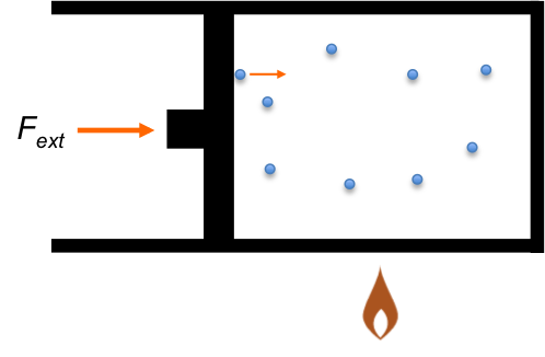
Show that  for a perfect gas (one that obeys the ideal gas law and exhibits a heat capacity that is independent of temperature) using the above diagram where
AC: reversible isothermal process
AB: reversible isochoric process
BC: reversible isobaric processes
Answer
The change in internal energy  from point A to C along the isotherm AC is zero for an ideal gas. Since is a state function, for the process AC and ABC is the same:

The change in internal energy for path ABC is:
+(U_B-U_A)=\Delta U_{BC}+\Delta U_{AB})
dT-p_1\int_{V_1}^{V_2}dV+\int_{T_A}^{T_B}C_V(T)dT)
Assuming and are constant over the temperature range,
-p_1(V_2-V_1)+C_V(T_B-T_A))
Since  and
and  , we have, after applying the ideal gas law,
-p_1\left(\frac{nRT_C}{p_1}-\frac{nRT_B}{p_1}\right)+C_V(T_B-T_C))
Rearranging gives

Previous article: Enthalpy