The analytical solution of the energy equation for lithium involves finding analytical expressions for all terms in eq94 using one-electron trial wavefunctions. Guess values are used for the variables in all the wavefunctions except one, e.g. . Eq94 is then minimised to obtain the solutions for E and
. The process is repeated until E and all
become invariant.
After removing and
due to spin orthogonality from eq94, we have
where
Our computation employs the following assumptions:
- The ground state of Li is described by a single Slater determinant.
- Eq113 is minimised iteratively via the restricted open-shell method, where the 1s orbital is doubly occupied with
, while the 2s orbital is singly occupied. Therefore, we can substitute eq56 in eq113, where
, to give
- The 2s Slater-type orbital
is derived via the Gram-Schmidt process, as the generic 2s Slater-type orbital is not orthogonal to the 1s Slater-type orbital.

Question
Using the normalised 1s Slater-type orbital and the un-normalised generic 2s Slater-type orbital
, derive
via the Gram-Schmidt process.
Answer
With reference to eq111, we have
where N’ is the normalisation constant.
Substituting and
in the above equation and integrating using the identity
(see this article for proof), and then normalising and rearranging the result, we have
where
Let’s evaluate the remaining terms in eq114, beginning with . Substituting eq116 in
and integrating,
Next, we evaluate , which is equal to
. Substituting eq116 and eq47 in
and integrating (refer to the integration procedure in this article), we have
Finally, we evaluate . Referencing the steps in integrating
, we have
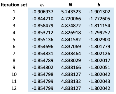
Substituting eq119, eq129, eq142 and the atomic number in eq114, we have the analytical expression of E, which is used in an iterative algorithm to determine the ground state of Li. The procedure involves setting up an iterative table in Excel as follows:
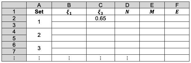
Cell C2 is the initial guess value of . Cell F2 contains the entire formula of the analytical expression of E, with links to B1, C1, D1 and E1. Cell D2 and E2 contain the formulae of N and M respectively, with links to B1 and C1. The formulae for B3, D3 and E3 are ‘=B2’, ‘=D2’ and ‘=E2’ respectively. To compute the first iteration set, we employ the Excel Solver application to minimise F2 with respect to B2, with the following settings:
Set objective: F2
To: Min
By changing variable cells: B2
Selecting a solving method: GRG Nonlinear
We then solve for F3 by changing the ‘Set objective’ field and ‘By changing variable cells’ field to D3 and C3 respectively. This procedure is repeated for subsequent iteration sets until the values of and
are invariant up to seven decimal points.
The results are as follows:
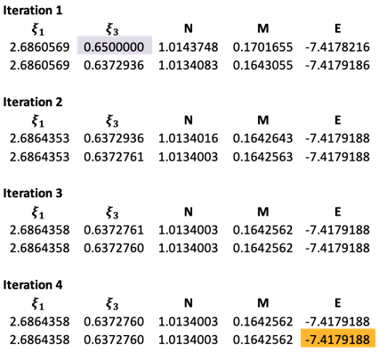
The final theoretical value of has a deviation of about 0.80% versus the experiment data of the ground state of Li.